Revisiting Land Remote Sensing Issues: Lessons Learned 30 years ago

Revisiting Land Remote Sensing Issues: Lessons Learned 30 years ago

Garik Gutman

Download PDF

1.     Introduction

Studying physical processes at the land surface from space require careful data processing to remove noise caused by atmospheric effects and artificial trends caused by drifts in sensor sensitivity and satellite orbit. Although some problems have been addressed, researchers handling long-term time series still encounter difficulties throughout the processing chain. Those include atmospheric effects and surface anisotropy, as well as distinguishing between true physical trends and data artifacts caused by instrument-related issues. This paper provides a brief overview of the data processing chain used to derive land surface variables, highlight persistent and often treacherous residual errors in compositing procedures and applying smoothing filters, and draw attention to key challenges that scientists continue to encounter when working with long-term time series of remote sensing data over land. The examples are based on the lessons learned from author’s research in the 1990s.

Advanced methodologies including Machine Learning algorithms and Artificial Intelligence approaches further resolve processing issues. Nevertheless, it is worth revisiting the traditional methods and analyze lessons learned during the past 30 years that may contribute to the development of modern, advanced algorithms.

2.  Processing chain for deriving land surface variables

Before deriving surface variables from visible, near-infrared, and infrared observations, several essential steps are routinely performed.

2.1  Geo-correction 

Registration is essentially the alignment of one image to another image of the same area, while geo-referencing (or rectification) is the alignment of an image to a map so that the image is planimetric, like the map. Pixel-by-pixel correction for topographic distortion is referred to as orthorectification.

2.2  Calibration   

The response of a sensor (in digital numbers DNs) represents the reflectance being measured at a particular wavelength and is the base of calibration procedure. What is to be calibrated is essentially a system of electronics that produces a signal to measure intensity variations of incoming spectroradiance. Most instrument calibration is in a laboratory setting. Calibration coefficients (to convert DNs to radiances) are usually supplied with data. The trouble is that often these coefficients may be outdated because of degradation of sensor sensitivity while onboard of a satellite (or even prior to the launch). This has been the case with AVHRR instruments onboard NOAA polar orbiting satellites that provide the basis of long-term series starting early 1980s. Efforts to correct the calibration coefficients with post-launch calibration, usually on bright surfaces, have been made. Reviews can be found, e.g., in Molling et al. (2010), Kalluri et al. (2021), Dech et al. (2021).

2.3  Cloud filtering 

Traditional methods for screening clouds in land surface studies included: thresholding of spectral ratios and differences; texture analysis (spatial coherence); tests on continuity (temporal coherence); and compositing (assuming that at least one observation is clear during the compositing period). However, recent reviews highlight a massive shift in cloud screening for AVHRR data away from static, rule-based threshold tests and toward probabilistic models and Deep Learning. While computationally fast, the traditional methods are highly sensitive to threshold settings and often misclassify complex or sub-pixel cloud boundaries. Instead of binary “cloudy/clear” screening, recent frameworks utilize probabilistic masking, providing continuous metrics to assess pixel-level confidence. Machine Learning, specifically Neural Networks approach, dynamically extract features across massive time-series, outperforming traditional multi-channel thresholds over bright land surfaces. Description of traditional methods can be found, e.g., in Chen et al. (2002), while advanced methods can be found in Karlsson (2025) and Bulgin et al. (2024).

2.4  Atmospheric correction      

This step consists of estimating atmospheric path radiance and view path transmittance and then solving for at-surface radiance. Vermote and Kotchenova (2008) provided detailed description of atmospheric corrections required to obtain at-surface radiance, ultimately deriving surface spectral reflectances. Briefly, the correction algorithm requires the knowledge of key atmospheric parameters, the most important for the visible range being aerosol optical thickness retrieved from data itself, and such aerosol characteristics as single scattering albedo, particle size distribution, and refractive index, prescribed by a selected aerosol model. For the infrared range, correction for water vapor is most critical with the input either derived from data itself or imported from independent sources.

2.5  Anisotropic correction

Typically, corrections rely on semi-empirical, kernel-driven bi-directional reflectance distribution function (BRDF) modeling, as originally introduced by Roujean et al. (1992). Model parameters are estimated from multiple observations of the same pixel at different angles and include temporal compositing, least-squares regression, and prior land-cover BRDF libraries. Other early approaches involved fitting empirical polynomial functions to aggregated observations across the available viewing geometries in the dataset (see, e.g., Gutman 1994), or using an independent dataset or model, such as in Gutman et al. (1989). Ultimately, in most methods observations are normalized to a common geometry.

2.6  Derivation of reflectances and temperatures

Following geo-correction, calibration, cloud screening and atmospheric and anisotropic corrections, spectral reflectances and brightness temperatures are determined, and vegetation indices are calculated. The subsequent level may involve the computation of surface physical variables such as albedo, skin temperature, vegetation fraction, leaf area index, and others.

Conversion of at-surface radiance to reflectance requires 3 more parameters: solar pathatmospheric transmittance (from model or measurements), exo-atmospheric solar spectral irradiance (known) and incident angle (from Digital Elevation Models) (Vermote and Kotchenova, 2008).

Skin temperatures are commonly derived using split-window techniques with surface emission either prescribed for observed land-cover or calculated based on derived vegetation characteristics from data itself (Sobrino et al. 1991; Sobrino and Cuenca, 1999).

3. Challenges of using composited images

In the 1990s (and sometimes even today), land surface studies have used so-called composite datasets created by selecting one data point in a certain time (compositing) period by employing an assumption that the clearest observation occurs when observed vegetation index is at its maximum (e.g. Holben 1986). While the assumption that compositing provides cloud-free observations holds true in some cases, it often fails, especially in persistently cloudy regions. Residual cloud contamination in composite datasets poses a significant challenge for non-remote sensing scientists, who may lack awareness of these processing issues and are primarily focused on analyzing the data to identify physical changes at the land surface.

Compositing procedures were developed in the early 1980s as a “quick & dirty” screening for atmospheric effects, including clouds, and fast data compression with much of the noise removed, which rendered a more “eye pleasing” viewing of image sequence, represented by mosaics of pixels from clearest cloud-free observations. Temporal pixel-by-pixel compositing were based on selecting the greenest pixel (in time and/or in space) based on a calculated ratio or difference between visible and near-infrared data or sometimes selecting the darkest (lowest reflectance) and/or warmest (highest temperature) pixel (see Sihlar et al. 1997).

Although atmospheric effects are largely reduced using, for example, the maximum value compositing based on Normalized Difference Vegetation Index (NDVI) (Holben 1986), quantitative results in many regions may be inaccurate because of residual cloud contamination, temporal atmospheric variability and varying sun-target-sensor geometry. Alternative methods to reduce noise in NDVI time series and retain more realistic NDVI values in time series included Best Index Slope Extraction algorithm (Viovy et al. 1991).

3.1 Improvement of composite imagery      

If researchers use a composite dataset, additional screening of NDVI composites can be based on a combined use of reflectance and temperature data associated with the composite NDVI image pixels (Gutman et al. 1994). A result of applying such a special post-composite screening algorithm is shown in Fig. 1 over a 2 deg x 2 deg area in Thailand during 1988-1989.  The profiles of screened and unscreened NDVI are almost identical during the dry season (December-April) when post-composite cloud filtering does not introduce much improvement. Large discrepancies in the monthly screened and unscreened averages, however, are clearly pronounced during the monsoon season.

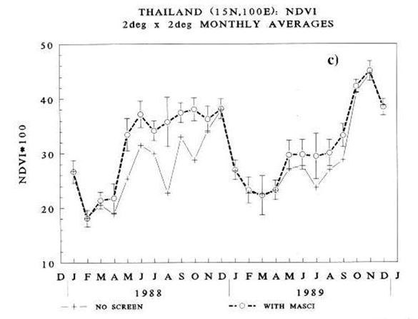
Figure 1. Temporal variability of NDVI averaged over an area in Thailand for two years: without screening (+) and with additional screening (o).

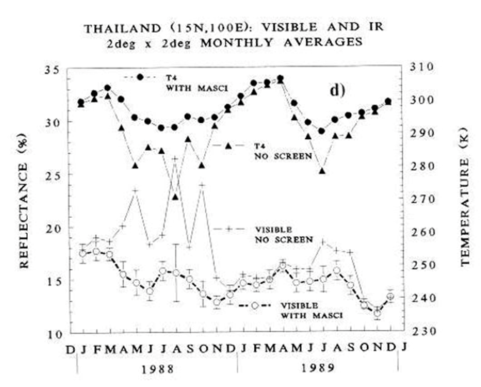
Figure 2. Same as in Figure 1 for visible reflectance without screening (+), with additional screening (o), and temperature without screening (triangles) and with additional screening (dots).

The NDVI discrepancies can be understood from Fig. 2, where the associated cold (low temperature) and bright (high reflectance) values reveal unscreened cloud contamination.

3.2 Dangers of applying smoothing filters to a cloud-contaminated data

Applying statistical filters, such as those described by van Dijk et al. (1987), to composited data without proper cloud screening can lead to inaccurate temporal profiles of vegetation indices. This occurs because the filter tends to fit most data points—which may be cloud-contaminated—while disregarding outliers. In regions with persistent cloud cover, such as during the monsoon season in Thailand, these outliers often correspond to the few cloud-free observations. Fig. 3 illustrates the impact of using a 5-point median filter on the original weekly NDVI composites. The resulting profile is clearly incorrect, as the filter relies on cloudy pixels for smoothing. Therefore, smoothing filters should only be applied after thorough physical filtering—such as the procedures described in section 3.1—to ensure data accuracy.

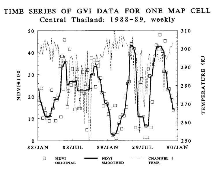
Figure 3. Variability of NDVI original data (squares), its fit by a 5-point median filter (solid curve) and the corresponding brightness temperature (dashed curve) in a 20 km x 20 km map cell in Thailand.

3.3. Potentially erroneous spatial distribution in the composite

        When observations are infrequent, such as those collected by a single Landsat sensor, compositing can risk producing an inaccurate spatial distribution of pixels within a mosaic. For example, imagine two neighboring agricultural areas during the growing season, with their NDVI values rising from 0.3 at the start of the month to 0.7 by month’s end. Suppose the first area is cloud-free only at the beginning of the month, while the second is cloud-free only at the end. The composite NDVI for the first field would be 0.3, and for the second, 0.7. Ideally, both areas should yield the same NDVI value by the end of the month but the resulting mosaic would misrepresent the true spatial distribution.

3.4 Sun-target-geometry effects

        Even after screening for clouds, cloud-free data require additional correction to account for bidirectional effects caused by the anisotropic nature of the land surface. This issue is less significant for sensors that consistently maintain near-nadir viewing angles; however, it can lead to misinterpretations when using scanning instruments with large orbital swaths, such as AVHRR, MODIS, or the MSI onboard Sentinel-2. The periodic fluctuations in reflectance, resulting from changes in sun-target-sensor geometry, were first observed in the 1980s (Gutman 1987), and their underlying cause became clear once the AVHRR scanning patterns were thoroughly understood.

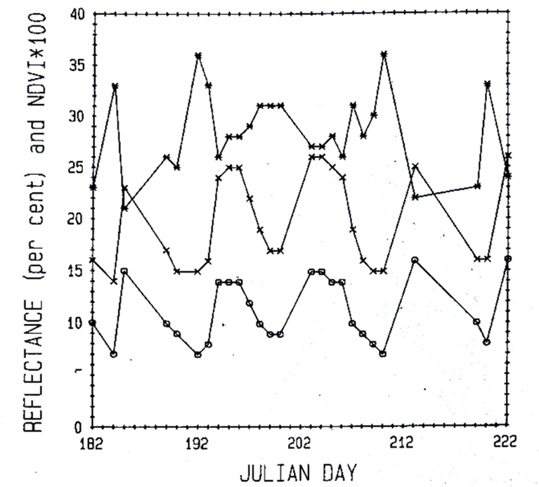
 Figure 4. Variability of AVHRR visible (o) and near-infrared (x) reflectances and NDVI (*) for one map cell in Kansas after cloud screening.

        Figure 4 illustrates the temporal variability of a cloud-free pixel in AVHRR data over an area in Kansas. Both visible and near-infrared reflectances fluctuate significantly, ranging from 60% to 100% relative variability, with a distinct periodicity. In contrast, NDVI shows much less regularity in variation, except for periodic spikes that occur at specific geometric configurations. Figure 5 helps interpret these effects: Panel 5a displays the 9-day saw-tooth periodicity of the solar zenith and sensor viewing angles, which correspond to the observations in Figure 4. Panel 5b provides a schematic view of the 9-day progression of these angles relative to the Earth’s surface target. The sun-target-sensor geometry affects reflectances depending on whether the area is viewed in the direction of the sun’s rays (backscatter) during one half of the 9-day cycle, or against the sun (forward scatter) during the other half. Typically, discontinuities appear at the seams between two stitched AVHRR orbits across a large region (not shown).

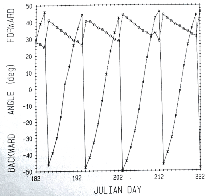
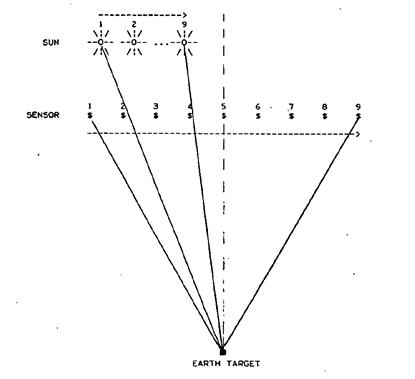
Figure 5. Left: (a) Periodicity of the viewing (x) and solar zenith (o) angles for one map cell associated with the observations in Fig. 4. Right (b): A schematic diagram of the 9-day periodicity in sun-target-sensor geometry of AVHRR scanner.

The origin of the 9-day cycle can be traced to the AVHRR’s orbital patterns, as illustrated in Fig. 6. Each day, the sensor completes 14 scanning orbits that cover the entire globe. However, these orbits are not perfectly in phase, so the N+14th orbit is offset from the Nth orbit by one-ninth of the orbital swath. This offset causes the orbits to realign (“get in phase”) every 9 days, resulting in the observed periodicity.

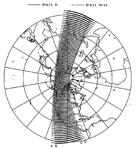
Figure 6. The AVHRR orbital patterns for the N^th and the N+14^th orbits.

The NDVI spikes (the upper jagged line marked by *) in Figure 4 can be explained by transitions between extreme forward scatter and extreme backscatter directions. These transitions occur when the difference between visible and near-infrared reflectances becomes most pronounced, as illustrated in Figure 7 (Gutman 1991) for a region in Kansas. Interestingly, this phenomenon sheds light on the extreme backscatter bias observed in weekly composites in the NOAA Global Vegetation Index dataset. This bias arises because compositing for that dataset relies on the maximum value of the simple differences between near-infrared and visible counts. In contrast, the NASA GIMMS NDVI dataset is constructed using the maximum NDVI value, which introduces a subtle forward viewing bias (see histograms in Gutman 1991).

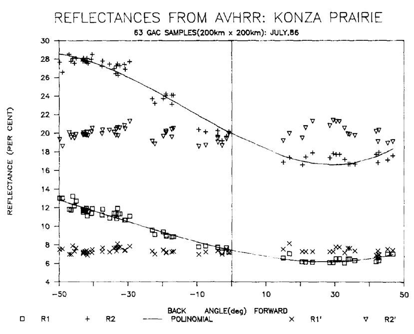
Figure 7. Variability from back to forward scatter direction of visible and near-infrared reflectance observations in Kansas area in July and their fit with polinomials (solid lines): visible uncorrected (squares), visible corrected (x), near-IR uncorrected (+) and corrected (triangles).

Mathematically, NDVI can be expressed as a function of r=R₂/R₁, called “simple ratio”. 

NDVI=(R₂-R₁)/(R₂+R₁)=(r-1)/(r+1)

The simple difference between near-IR and visible reflectance, called Difference Vegetation Index (DVI) can be expressed as follows:

DVI=(R₂-R₁)=R₁ (r-1)

            Thus, the DVI is a function of two variables: the visible reflectance and the ratio. The NDVI, on the other hand, is a function of one variable – the ratio. As a result, the points at which the DVI reaches its maximum are not the same as those for the NDVI. The DVI peaks in the extreme backscatter when R1 is at its highest value. This distinction clarifies the differences observed between the two composite datasets: the NOAA GVI and the NASA GIMMS (see Gutman et al. 2021).

4.    Long-term monitoring challenges

4.1 Satellite sensor degradation

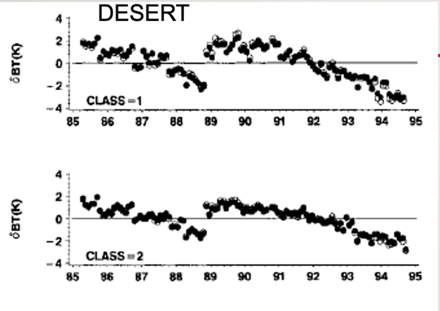
Processing long-term data introduces additional challenges. Satellite sensors frequently degrade over time, so either continuous onboard calibration is conducted, or post-launch calibration coefficients are applied. Without these measures, comparing derived variables across different time periods may be unreliable. Moreover, long-term observations typically involve stitching time series from multiple satellites, which can introduce uncertainty during satellite replacement. Even after correcting each satellite’s time series for sensor degradation, residual errors may cause discontinuities that could lead researchers to incorrect interpretations.  Fig. 8 shows time series of anomalies of AVHRR visible and near-IR reflectances globally averaged over all points classified as “deserts” (Gutman 1999).

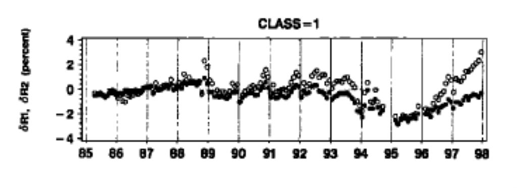
Figure 8. Time series of anomalies of visible (dots) and near-IR (circles) for all desert data lumped into one class and averaged (from Gutman 1999).

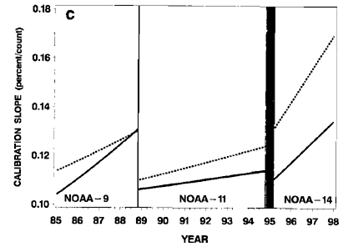
Figure 9. Calibration slopes in time for NOAA-9, -11 and -14.

There have been numerous efforts to recalibrate all NOAA AVHRR data and detrend the time series. Usually, bright area targets have been used for vicarious post-launch calibration. Sometimes global approaches were employed, e.g. Brest and Rossow (1992) or Gutman (1999). Molling et al. (2010) reviewed most of the recalibration methodologies attempting to find a consensus.

4.2 Satellite orbit drift

Orbital drift can cause apparent changes in reflectance and temperature measurements, which may be mistakenly interpreted as actual shifts in Earth’s surface conditions and lead to incorrect conclusions about environmental trends. In fact, these top-of-atmosphere variations are the result of altered illumination and increased downwelling path lengths, which progressively affect atmospheric influences on AVHRR observations and produce discontinuities (Gutman 1999).

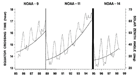
Figure 10. Drift and discontinuity in observational local time (solid line) and solar zenith angle (dashed line).

During the 1990s, observed trends in NOAA satellite data were largely the result of satellites drifting to later equator crossing times. This drift introduced trends and discontinuities in the solar zenith angle of observation (see Fig. 10), affecting both reflectance and temperature measurements (due to progressively later observation times). To ensure reliable land surface monitoring, it is crucial to remove these spurious trends and discontinuities occurring during satellite transitions.

Changes in illumination over time also introduce trends in anisotropic effects, such as shadowing. Temperature time series are influenced not only by shifts in the local observation time but also by variations in sunlit and shaded conditions, posing a significant challenge for the long-term monitoring of thermal observations. Figure 11 illustrates the time series of anomalies in AVHRR-observed brightness temperatures, grouped into the “desert” and “semi-arid” classes, during the NOAA-9 and NOAA-11 periods. Each period exhibits an overall global “cooling” trend for each satellite observational period, with a noticeable discontinuity corresponding to the satellite transition from NOAA-9 to -11.

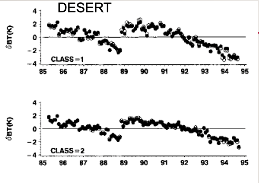
Figure 11. Trends in brightness temperatures’ anomalies averaged over “desert” and “semi-arid” classes for the NOAA-9 and -11 satellite time periods.

These artificial trends can confuse—or worse, mislead—physical scientists who are unaware of underlying data issues. For this reason, remote sensing specialists working with long-term datasets have a responsibility to remove these distortions as thoroughly as possible, ensuring that genuine land surface anomalies across various regions are accurately detected and monitored. Below are prominent initiatives in Europe, the USA, and Asia dedicated to reprocessing long-term AVHRR time series:

1. The TIMELINE 1km AVHRR NDVI Product: DLR with contribution from CESBIO
   • Analysis of 30-year seasonal trends (spring, summer, autumn) for European and North African land cover types.
2. Land Long Term Data Record (LTDR) @NASA, USA
   • Reprocessing of 4 decades of Global Area Coverage (GAC) data to produce consistent daily surface reflectance and vegetation indices (NDVI/EVI2) at 0.05-degree resolution.        
3. The Global Land Surface Satellite (GLASS) AVHRR @ Center for Global ChangeData Processing and Analysis at Beijing Normal University, China
   • Generation of 8-day normalized reflectance and vegetation products using refined reconstruction methods to reduce noise.

4.       Conclusions 

This paper revisited the pertinent issues in land remote sensing for proper processing the available data before they are used in land surface applications. Without thorough pre-processing, long-term data series from AVHRR and its followers – MODIS and VIIRS – onboard polar-orbiting satellites would suffer from inconsistencies, spatial inaccuracies, and atmospheric distortions. Critical procedures, including calibration, geolocation, atmospheric correction, cloud masking and harmonization, are essential for ensuring that reflectance and temperature data are accurate, comparable, and reliable for scientific analysis. These datasets provide unparalleled global coverage and continuity spanning multiple decades, making them indispensable for analyzing and interpreting environmental changes on a regional basis and applications in forest, agriculture, and urban sectors, as well as Earth’s system modeling.

        The primary aim of this paper is to let early to mid-career remote scientists aware of the fundamental challenges inherent in data acquired from passive optical sensors, particularly those with coarse spatial resolution. This brief overview highlights critical issues and provides essential references to comprehensive reviews of traditional methods and the latest, advanced methods for processing these data.

Autor Contributions

Garik Gutman: Funding acquisition, Project administration, Resources, Supervision, Investigation, Conceptualization, Methodology, Writing – Review & Editing.

Declaration of Competing Interest

The author declare that they have no known competing financial interests or personal relationships that could have appeared to influence the work reported in this paper.

Acknowledgments

The author would like to thank Prof. José Sobrino for the invitation to the RAQRS VIII symposium and encouragement to write this paper. The author thank the associate editor and the reviewers for their systematic review and valuable comments.

Funding

This research was funded by NASA LCLUC Program.

References

Aksakal, S. K., Neuhaus, C., Baltsavias, E., Schindler, K., 2015. Geometric Quality Analysis of AVHRR Orthoimages. Remote Sensing, 7(3), 3293-3319. https://doi.org/10.3390/rs70303293

Asam, S., Eisfelder, C., Hirner, A., Reiners, P., Holzwarth, S., Bachmann, M., 2023. AVHRR NDVI Compositing Method Comparison and Generation of Multi-Decadal Time Series—A TIMELINE Thematic Processor. Remote Sensing, 15(6), 1631. https://doi.org/10.3390/rs15061631

Bulgin, C. E. , R. I. Maidment, D. Ghent,  C. J. Merchant, 2024. Stability of cloud detection methods for Land Surface Temperature (LST) Climate Data Records (CDRs), Remote Sensing of Environment, 315, 114440, ISSN 0034-4257, https://doi.org/10.1016/j.rse.2024.114440.

Brest, C. L., and W. B. Rossow, 1992. “Radiometric calibration and monitoring of NOAA AVHRR data for ISCCP,” Int. J. Remote Sens., 13, 235-273.

Chen, P.Y., R. Srinivasan, G. Fedosejevs, B. Narasimhan. An automated cloud detection method for daily NOAA-14 AVHRR data for Texas, USA, International Journal of Remote Sensing, 23, 2002, 2939-2950 (online 2010).

Cihlar, J., D. Manak, and M. D’Iorio, 1997. “Evaluation of compositing algorithms for AVHRR data over land,” IEEE Transactions on Geoscience and Remote Sensing, vol. 35, no. 5, pp. 1380-1393.

Dech, S., Holzwarth, S., Asam, S., Andresen, T., Bachmann, M., Boettcher, M., Dietz, A., Eisfelder, C., Frey, C., Gesell, G., et al., 2021. “Potential and Challenges of Harmonizing 40 Years of AVHRR Data: The TIMELINE Experience.” (“Potential and Challenges of Harmonizing 40 Years of AVHRR Data: The …”) Remote Sensing, 13(18), 3618. https://doi.org/10.3390/rs13183618.

Gutman, G., Gruber, A., Tarpley, D., Taylor, R., 1989. Application of angular models to AVHRR data for determination of the clear-sky planetary albedo over land surfaces. Journal of Geophysical Research, 94(D7), 9959-9970. https://doi.org/10.1029/JD094iD07p09959

Gutman, G., 1991. Vegetation indices from AVHRR: An update and future prospects. Remote Sensing of Environment, 35, 121-136.

Gutman, G., 1994. Normalization of multi-annual global AVHRR reflectance data over land surfaces to common sun-target-sensor geometry. Advances in Space Research, 14(1), 121-124.

Gutman, G., Ignatov, A., Olson, S., 1994. Towards better quality of AVHRR composite images over land: Reduction of cloud contamination. Remote Sensing of Environment, 50, 134-148.

Gutman, G., 1999. On the use of long-term global data of land reflectances and vegetation indices derived from the Advanced Very High Resolution Radiometer. Journal of Geophysical Research, 104, 6241-6255.

Gutman, G., Skakun, S., Gitelson, A., 2021. Revisiting the use of red and near-infrared reflectances in vegetation studies and numerical climate models. Science of Remote Sensing, 4, 100025.

Holben, B. N., 1986. Characteristics of maximum-value composite images from temporal AVHRR data. International Journal of Remote Sensing, 7(11), 1417-1434.

Julien, Y., Sobrino, J.A. 2012. Correcting Long Term Data Record V3 estimated LST from orbital drift effects. Remote Sensing of Environment, 123, 207- 219. https://doi.org/10.1016/j.rse.2012.03.016

Kalluri, S., Cao, C., Heidinger, A., Ignatov, A., Key, J., Smith, T., 2021. The Advanced Very High Resolution Radiometer: Contributing to Earth Observations for over 40 Years. Bulletin of the American Meteorological Society, 102(2), E351–E366.

Karlsson, K.-G., Håkansson, N., Eliasson, S., Wolters, E., Scheirer, R., 2025. Extension of AVHRR-based climate data records: exploring ways to simulate AVHRR radiances from Suomi NPP VIIRS data. Atmospheric Measurement Techniques, 18, 3833–3855. https://doi.org/10.5194/amt-18-3833-2025

Molling, C. C., Heidinger, A. K., Straka, W. C., III, & Wu, X. (2010). Calibrations for AVHRR channels 1 and 2: Review and path towards consensus. International Journal of Remote Sensing, 31(24), 6519-6540. 

Singh, R., Pal, M., Biswas, M., 2025. Cloud Detection Methods for Optical Satellite Imagery: A Comprehensive Review. Geomatics, 5(3), 27. https://doi.org/10.3390/geomatics5030027

Sobrino, J. A., Coll, C., Caselles, V., 1991. Atmospheric correction for land surface temperature using NOAA-11 AVHRR channels 4 and 5. Remote Sensing of Environment, 38(1), 19-34.

Sobrino, J. A., Raissouni, J., 2000. Toward remote sensing methods for land cover dynamic monitoring: Application to Morocco. International Journal of Remote Sensing, 21(2), 353-366.

van Dijk, A., Callis, S., Sakamoto, C. and Decker, W. 1987. Smoothing vegetation index profiles: An alternative method for reducing radiometric disturbance in NOAA/AVHRR data. Photogrammetric Engineering and Remote Sensing, 53, 1059-1067.

Vermote, E. F., Kotchenova, S. Y., 2008. Atmospheric correction for the monitoring of land surfaces. Journal of Geophysical Research: Atmospheres, 113(D23), D23S90. https://doi.org/10.1029/2007JD009662

Viovy, N., Arino, O., Belward, A. S., 1992. The Best Index Slope Extraction (BISE): A method for reducing noise in NDVI time-series. International Journal of Remote Sensing, 13(8), 1585–1590. https://doi.org/10.1080/01431169208904212

Publisher’s Note

The statements, opinions and data contained in all publications are solely those of the individual author(s) and contributor(s) and not of Recent Advances S.L. and/or the editor(s). Recent Advances S.L. and/or the editor(s) disclaim responsability for any injury to people or property resulting from any ideas, methods, instructions or products referred to in the content.