


Long-term and short-term estimations of snow water availability from the Barasona reservoir
Lucas López
1,2*,María José Escorihuela

1
- isardSAT, Spain.
- Autonomous University of Barcelona, Spain.
* Author to whom correspondence should be addressed.


Abstract
The Barasona reservoir is one of the three main water supplies for the Aragon and Catalonia Irrigation District the principal provider for 98.000 ha, including 37 municipalities and thousands of agricultural holdings and livestock farms. Thus, it is of great interest to have a correct understanding of the reservoir’s hydrological processes. In this study we combine remote sensing and in-situ data to estimate the amount of water in the form of snow available for the Barasona reservoir and predict its input flow, in addition to estimate the dates of the beginning and ending of thaw. First, we estimate the snow cover area (SCA) from MODIS and Sentinel 2. For Landsat 8, an equivalent algorithm is implemented to derive the snow cover. The result is a time series of SCA from 2009 to 2023. With this SCA together with snow height measured at the catchment we estimate the snow water equivalent (SWE). All this data along with in-situ information from weather stations is fed to an AI model that predicts the Barasona reservoir input flow in the short term. The base model achieved an accuracy of R2 = 0.691. If the flow from previous days was inputted as a variable, the performance increased to R2 = 0.781. Regarding long-term predictions, the estimated dates of the beginning and end of snowmelt are March 23 and May 26, with two weeks of standard deviation. The SWE available shows large inter-annual variability, ranging from 48.82hm3 during years of drought to 228.77hm3 when snow is abundant, with an average of 120.27hm3, and a standard deviation of 58.15hm3.Keywords
Snow Water Equivalent, Pyrenees, Machine Learning, Irrigation, Reservoir1. Introduction
In semi-arid climates, accumulated water in the form of snow at the mountains is an important asset, especially for agriculture, which in regions like the Mediterranean consumes on average a 69% of all water supply (Malek & Verburg, 2017; FAO, 2016). In fact, the Mediterranean is recognized by several studies as one of the most susceptible regions to climatic change in the following years (Alcamo et al., 2007; Ulbrich et al. 2006). Since mountain water resources are highly dependent on environmental fluctuations, alterations induced by global warming could have a great impact on their quantity and availability and thus in hydrologic management.
The estimation of the SWE available at a given region and its subsequent discharge can be performed by the means of either physical or empirical models. Physical models work by simulating the dynamics of hydrological phenomena like snow accumulation, snow sublimation, surface energy balance, snow melting and eventually catchment runoff, amongst others. For this, a large number of inputs regarding meteorological data, soil and canopy information and other environmental conditions are usually necessary. These models also usually present a high computational cost. Examples of these type of models are the CROCUS model (Vionnet et al., 2012), that simulates the time and space dynamics of snowpack and can be potentially coupled with atmospheric models, or the Soil and Water Assessment Tool (Arnold et al., 1988), a continuous-time, semi-distributed, small watershed to river basin-scale model simulating the quality and quantity of surface and ground water. Given the fixed specific inputs of this type of models, the inclusion of remote sensing data is not always viable unless some additional modification is added. For example, in Zhao et al. (2022), the SWAT model was modified to include, among other changes, the snow depth derived from passive microwave remote sensing data and temperature in the seasonal snowmelt area, which resulted in an improvement in the estimation of the snowmelt run-off of the Baishan basin in Northeast China.
Empirical models, on the other hand, do not consider the physical processes that take place at the studied region, but rather depend entirely on field data and observations collected in situ. Regression analysis techniques would fall under this category. An example of this would be the Base Difference Model developed by Veiga et al. (2014), that predicted the flow of the Bow River at Calgary, Canada during the colder months of the year thanks to the observed offset between measurements at other upstream flow gauges.
Inside this same group of data-driven models, a methodology known as the Long Short-Term memory (LSTM) network from the family of Machine Learning (ML) predictors can also be found. The LSTM model (Hochreiter & Schmidhuber, 1997; Gers et al., 2000) belongs to the category of recurrent neural networks (RNN), a type of neural network specialized in dealing with sequential data that can be especially useful when processing time series. As of right now, it is one of the most popular ML models because of its capability of dealing with the vanishing gradient problem, an issue that hinders other RNNs by slowing down the learning process and causing the network to miss the long-term dependencies.
This type of methodology is easy to implement, flexible, and has proven to be well-suited for predicting highly non-linear variables such as reservoir inflow. For example, in Herbert et al. (2021), several models including some based on the LSTM network are used to predict the long-term behavior of streamflow in Utah. In Song et al. (2022), the LSTM model is applied to forecast the SWE dynamics in different sites of the western United States. In a similar manner, we will try to see if this methodology allows us to determine the river flow in the short term in a precise way using available data at a given region of interest.
The Pyrenees and the Ebro River basin are a good example of a region that can be affected by climate change, as mentioned above. Between the Pyrenees and the Ebro river, a large number of irrigation districts can be found, and several reservoirs have been developed to properly manage water resources. During these last years, the Pyrenees have suffered several drought episodes, that have severely affected not only the mountain system itself, but also the regions that depend on its water supply, both economically and ecologically (Gazol et al., 2020; Reynaud, 2006). With global warming, and the consequences it entails, the duration and severity of these events will only increase.
The organism that manages all these reservoirs at a basin level is the “Confederación Hidrográfica del Ebro”, who is in charge of regulating and maintaining their water discharge to the hydrographical basin of the Ebro. During dry periods, it oversees the evaluation of the drought conditions, and emergency water allocation. It also processes and distributes the information extracted from the measurement network located at the catchment. The data they provide with respect to snow comes from the “Evaluación de los Recursos Hídricos procedentes de Innivación” (ERHIN) program, dedicated to quantifying these types of resources.
Recently, there has been an increase in the interest of acquiring higher precision data in regard to the available water resources and snow volume for the Ebro basin, with specific information as to when the fusion would begin (Quiroga et al. 2010, Linés et al., 2018). The reason for this is that the snow water volume that will eventually reach the reservoir during a year is basically determined by the beginning of thaw, so it represents a minimum water volume available that does not depend on future meteorological events, which is crucial for decision-making to the irrigation community.
Water resource information is usually extracted from hydrological and meteorological stations at the basin level. Remote sensing data provides a different source of information that can enrich the measurements from the in-situ instruments, optimizing the decisions taken by the corresponding managing organization so that water is properly distributed with minimal waste, which benefits not only the agricultural community, but also the environment. Thus, the objective of this study is to develop a methodology to estimate, using remote sensing data combined with in situ information, the snow water volume available and the subsequent discharge for a given reservoir basin.
We will focus on estimations at two time scales: i) Forecast in the long term the amount of water that the reservoir will receive during snowmelt and its starting period; and ii) Develop an AI-based neural network model that will allow to predict a reservoir river flow at a finer time resolution.
We will develop our methodology for the Ésera River basin and the Barasona reservoir, located at the Central Pyrenees. It is one of the main irrigation water suppliers for the “Canal de Aragón y Catalunya”, which consists in around 98.000 ha; and the object of intensive supervision by the “Comunidad General de Regantes” (CGR-CAyC), who manage its distribution of water to the 131 irrigation districts downstream the reservoir. Because of its importance, decisions regarding the reservoir’s discharge need to be regularly made to maximize the profitability of the resources available. For this purpose, water managers require as much information as possible with respect to the quantity and availability of water at the basin.
2. Materials and Study Area
2.1 Study Area
The Barasona reservoir is a mountain reservoir located North of the Spanish province of Huesca. With a storage capacity of 92.20 hm3, it collects water descending from the Pyrenees system by means of a gravity dam for irrigation and energy supply purposes. Its construction began in 1929 and was finished 3 years later in 1932, causing the permanent flooding of the village of Barasona, to which the reservoir owes its name. Its basin is managed by the “Confederación Hidrográfica del Ebro” (CHE), and it is one of the main water sources for the “Canal de Aragón y Catalunya” (CAyC), which is the principal provider for a total 98.000 ha, including 37 municipalities and thousands of agricultural holdings and livestock farms (CHE, n.d., CAyC, n.d.). Amongst the main crops that receive water from it are fruit trees (apple, nectarine, peach and pear), cereals (maize, alfalfa and barley) and grape vineyards.
The water that feeds the reservoir comes from two main rivers inside the basin: the Ésera river and the Isábena river. The Ésera is the river with the largest amount of water flow (812 hm3 of yearly average water flow) from the two. Its source can be found at 2500 m of altitude. The river extends 77 km until it reaches the reservoir’s lake (CHE, 2002a). The Isábena river, on the other hand, has its source at 2400 m above sea level, and travels 58 km until it merges with the Ésera about 2 km before reaching the dam (CHE, 2002b), delivering 194.7 hm3 yearly. Several other small streams can also be found at the region, that eventually join one of these two main rivers. The Ésera river water is also accumulated along its course at several points, creating small artificial lakes. At the higher altitudes of the reservoir basin, several mountain lakes can also be found. These lakes of glacial origin are known as known as “Ibons”, and are unconnected to any of the rivers. There is also a karst system at the northern sections of the region where water is drained underground to eventually join the Garonne River (Palazón & Navas, 2016).
The climate of the catchment is mountainous, presenting precipitation and temperature gradients from North to South due to the complex topography of the region and the great altitude variability; but also from West to East, depending on the proximity of the Atlantic Ocean and the Mediterranean Sea. At the lower sectors of the basin, temperatures can range from 30ºC to less than 0ºC throughout the seasons, with an average yearly temperature of around 15ºC. At regions of more altitude, the average descends to around 7ºC, and even less (<4ºC) for the higher peaks. Precipitations are more abundant in zones closer to the mountains (of around >2000 mm of annual rainfall, compared to around 1000 mm at the reservoir outlet), and usually take place during spring and autumn, with a small decrease during summer (except for sporadic rainstorms). In the winter, they take the form of snow and hail due to the low temperatures, especially at the North.
2.2 Materials
2.2.1. Remote sensing data
The main source of information regarding snow coverage over the region of interest is satellite remote sensing. MODIS Snow Cover L3 Global 500m Grid products (NASA, n.d.), Sentinel 2 snow products from Theia (Theia, n.d.), and Landsat 8 Collection 2 Level 2 images (USGS, n.d) acquired between September 2009 and August 2023 are used for this study. MODIS data provides daily information regarding the percentage of snow cover within a 500 m resolution grid. The Theia products used are binary snow cover maps that indicate the presence of snow at a 20m resolution, provided at a frequency of 2-3 days. The combination of these three sources of information allows us to take profit of the high temporal frequency of MODIS and the high spatial resolution of Landsat and Sentinel.
While these two products already provide the necessary snow cover information, an adaptation of the methods described in Gascoin et al. (2019) has been implemented to retrieve the SCA from the Landsat 8 images. These are the same procedures used to generate the Sentinel 2 snow products from Theia. The algorithm takes the Normalized Difference Snow Index (NDSI) and other spectral bands and combines them with a Digital Elevation Model (DEM) that we obtained from the Shuttle Radar Topography Mission to retrieve the snow cover from every pixel. Cloud information is extracted from the Pixel Quality Assessment band from Landsat products and is processed to obtain a definitive SCA map.
Because all the abovementioned products are based on optical data, the presence of clouds (a frequent situation in mountain areas) is translated into a lack of data.
Regarding MODIS data gaps, we can take advantage of the fact that, for almost every day of the year, we have two available images of the region from the two satellites (Terra and Aqua) equipped with the instrument. Thus, we can perform a superposition of these two sources. For this, we create a new combined image, where whenever there is a cloud pixel in one of them, we take the value that is available in the other. If the pixel is labelled as cloud in both images, we leave it empty. In the case where both images differ in the value of a non-cloudy pixel, we get the average between the measured value at both satellites.
A particular processing has been designed to temporally fill cloud induced data gaps. There are several days where, although a satellite image is available, the cloud cover value renders the image unusable for our purposes. To deal with this issue, we perform a linear temporal interpolation at the pixel scale. This interpolation is performed in batches, each corresponding to a single hydrological year. The process is also done separately for MODIS and for both Sentinel 2 and Landsat 8, since the difference in resolution between the first and the last two is considerably large. The results from year 2018-2019 are shown as an example in Figure 1.

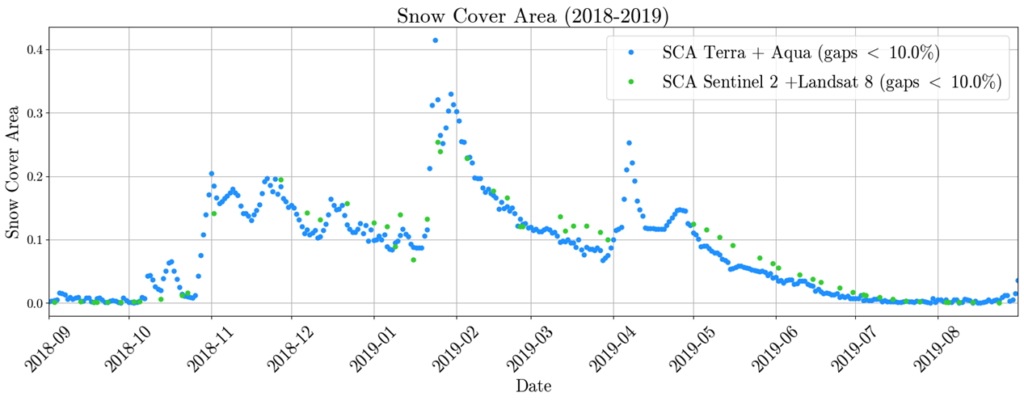
Figure 1: Snow cover area evolution over time for MODIS Terra+Aqua and Sentinel 2+Landsat 8 after the pixel-by-pixel temporal interpolation for year 2018-2019.
2.2.2. In situ data
In-situ information from the area of interest is collected by different sensors located across the region. There is a weather station located at the reservoir that provides not only meteorological data (humidity, atmospheric pressure, wind, sun irradiation, temperature and precipitation) but also information regarding the input and output flow of the reservoir. Then, eight rain gauges, five temperature stations, and four river gauges can be found throughout the basin, from which we extract precipitation and temperature information. We also obtained the measured snow height from two snow gauges at Eriste (1930 m) and La Besurta (2350 m) of altitude. In Figure 2, a visual summary of the information collected at every point is displayed on top of the DEM. The source for all this data is the Automatic Hydrologic Information System (SAIH), managed by the CHE. All the data used has a daily frequency, except for temperature, which is provided in 15-minute intervals.

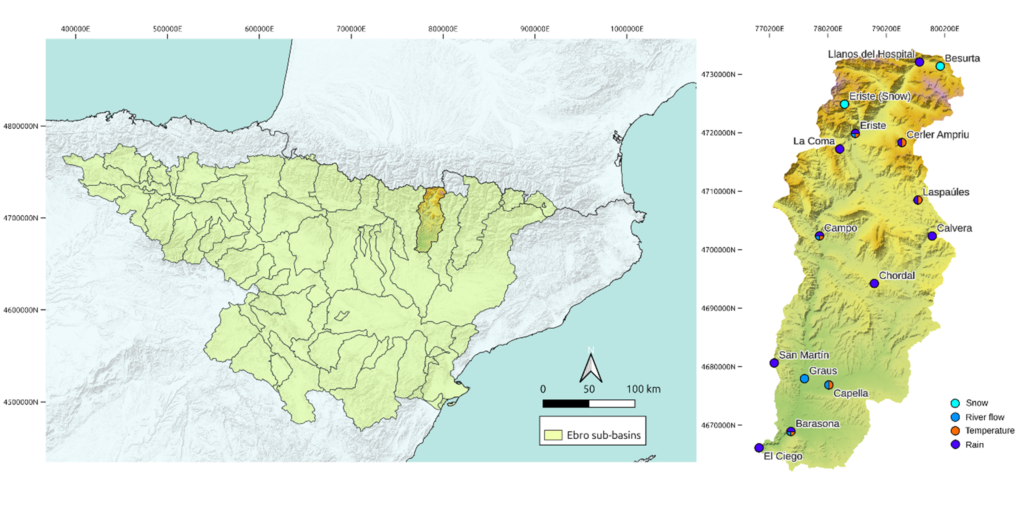
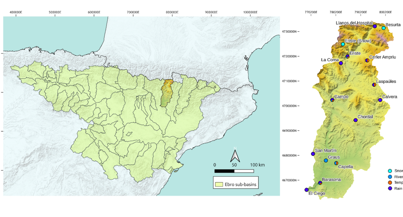
Figure 2: Left: Location of the Ésera sub-basin within the Ebro basin (highlighted in green). Right: Location every sensor across the region of interest. Orange is for temperature sensing, purple is for precipitations, blue is for river flow, and cyan is for snow. Coordinates (in meters) use the UTM zone 30N reference system.
The remote sensing data introduced in Section 2.2.1. presents highly accurate spatial information at every point of the catchment. In contrast, the in-situ data is a collection of time series extracted from different positions at the region of interest. In an effort to retain some of the spatial significance that is implicit in the geographical location of the different sensors, we have devised, for temperature and precipitation, a method to extend this data to the whole region and reprocess it so that it applies to the whole basin.
To extend the information from the temperature sensors to the rest of the basin, we use the concept of lapse rate, which is the rate at which atmospheric temperature changes with height (Jacobson, M. Z., 2005). Between the altitudes at which the weather stations are located, we perform a piece-wise interpolation that yields a corresponding estimation of the lapse rate of the basin every fifteen minutes. The slopes at the extremes of the interpolation are extended to the rest of altitudes that are not in between measuring stations. Then, using the DEM, we can infer the temperature at every position of the basin. Figure 3 provides an example of the process applied to compute the lapse rate, and the resulting extended temperature map. Looking at it, we notice that most of the sensors are located at the valleys of the region. The temperatures at the highest peaks, where temperature data is more relevant in regard to snowmelt, have needed to be extrapolated. Nevertheless, the presence of the stations allows us to detect variations of the lapse rate along with altitude, that would have otherwise been missed if a constant lapse rate had been used.

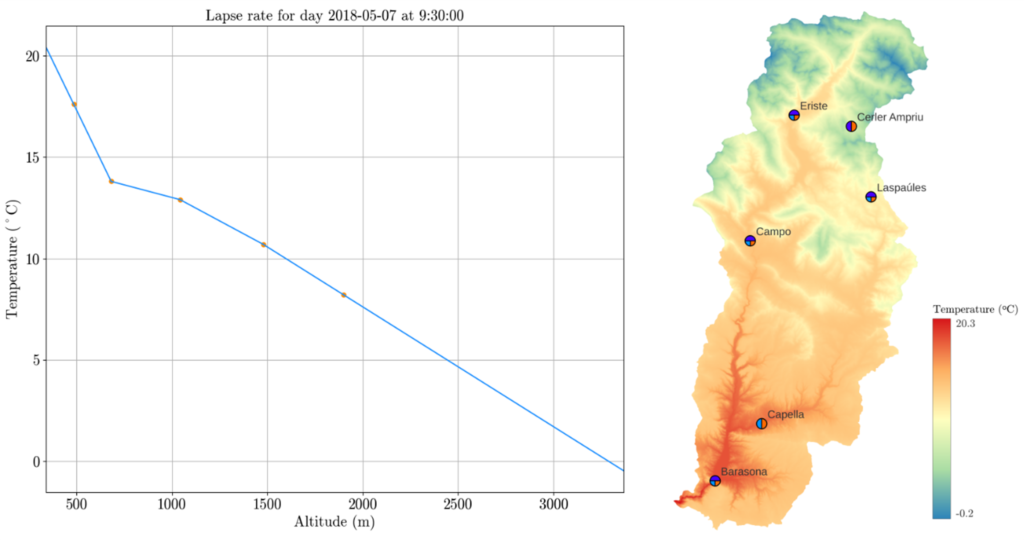
Figure 3: Left: Estimated piece-wise lapse rate by interpolating and extrapolating the available data from the sensors for the 7th of May of 2018, at 9:30 A.M. The limits of the x-axis are the minimum and maximum height of the basin. Right: Corresponding temperature map.
With respect to rainfall data, to interpolate it from the rain gauges to the rest of the basin, we make use of the notion of Thiessen polygons. A Thiessen polygon is a subdivision of the plane defined around a given point from a sample of points, so that any location inside the polygon is closer to that point than any of the other sample points (ESRI, n.d.). In this case, the positions of the different rain gauges are used as the points required to define a surrounding area that we assume shares the same characteristics as those measured at the rain gauge.
3. Methodology
During this section, we describe the procedures that have been applied to achieve the results of our study. First, we present the methodology used to derive the snow water volume from the snow cover area maps and the snow gauges data. Then, we explain the theoretical basis for the computation of what we call “short-term” and “long-term” predictions. Short term predictions refer to forecasts of the Barasona reservoir input flow that extend a short period of time into the future, one day in our case. These short-term predictions could be relevant for the management of the dam water level at the reservoir on a day-to-day basis. Moreover, we will define as “long-term predictions” those predictions regarding the total amount of water that will be collected at the reservoir throughout the year. Long-term predictions are useful for water managers to organize the distribution of water to the irrigation districts downstream, who in turn will be able to assess the type and quantity of crops that will be grown that year.
These long-term predictions will be a rough estimate extracted from a global analysis of the yearly behavior of the measured variables. Then, for the “short-term predictions” we will use a neural network model where a training-test split will be defined to properly assess the accuracy of our predictions.
3.1. SWE calculation
The basis of the calculation of the snow volume is the concept of minimum elevation of the snow cover , which is the lowest altitude at which snow can be found. For a given day, we assume that the snow height for all pixels at an altitude of is 0; and that all pixels at the same altitude share the same snow height. While these assumptions might not be necessarily always true, there is no other source of snow height information to our disposal. This allows us to perform an interpolation for the snow height for the whole basin using the two snow gauges. For all those pixels below , the snow height is assumed to be 0. For pixels above the Eriste snow gauge (at 2350 m), we perform an extrapolation of the values obtained in the interpolation. The area where the height is being extrapolated is only of 156 km2 (a 10% of the region), so this assumption does not have a large impact. Equation 1 summarizes the snow height interpolation applied. A schematic representation of the process is displayed in Figure 4.



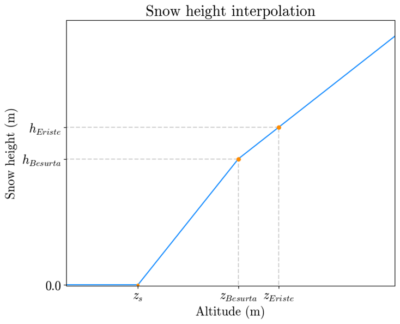
Figure 4: Schematic representation of the interpolation process used to infer the snow height at every point of the basin.
To obtain the snow volume from this, we only need to multiply the snow height at a given pixel times the size of the pixel , times the snow cover fraction value extracted from a given snow map, scaled from 0 to 1. To go from snow volume to water equivalent volume we need then to multiply this again by a factor that considers the change of volume from snow to water. The exact value of this parameter depends on the porosity of the snow and change of density from ice to water. We obtained this value from the literature (Muskett, 2012; Patterson, 1994; Fassnacht et al. 2010; HEC-HMS, n.d.), where different snow density measurement campaigns yield that , as a middle term conversion factor between snowpack and freshly fallen snow densities. The definitive formula for the total SWE can be seen in Equation 2:


With this equation, the amount of water in the form of snow at a given day where a satellite image is available can be estimated. For this, we use the snow maps that were presented previously in Section 2.2.1. In those days where we have two different sources of snow area cover (one image from MODIS and another from Landsat combined with Sentinel), we average the two possible values obtained. The temporal frequency of the snow water volume data is thus fully determined by the availability of MODIS or Landsat imagery.
In Figure 5 we observe as an example the snow height dynamics for the year 2018-2019 after the temporal interpolation on the top, and the computed SWE volume time evolution for the same year on the bottom. The correlation between the curves is quite visible. A maximum in February, that was also present in the SCA (see Figure 2) can also be observed here. Notice too two relative maxima in the snow height during spring, around April and May, that have been captured in the SWE curve, but were actually also hinted in Figure 2. This last fact would point out to the idea that the processing of the area information has been done correctly, which further confirms the validity of the SWE data computed. The rest of the computed snow volume curves can be found in Figure 6.

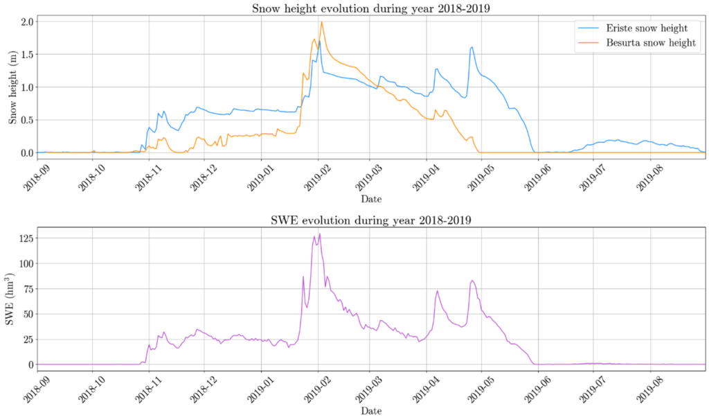
Figure 5: Top: Snow height post-interpolation during the year 2018-2019. Bottom: SWE time evolution during year the 2018-2019.
As we have seen, this simple methodology that we implemented allows us to obtain a consistent time series of the snow volume despite only being two snow gauges across the basin. But this simplicity comes at the cost of not being able to consider other variables that have a significant effect on snow accumulation distribution, such as the wind speed and direction during snow events, or local variations in snow density due to external factors.

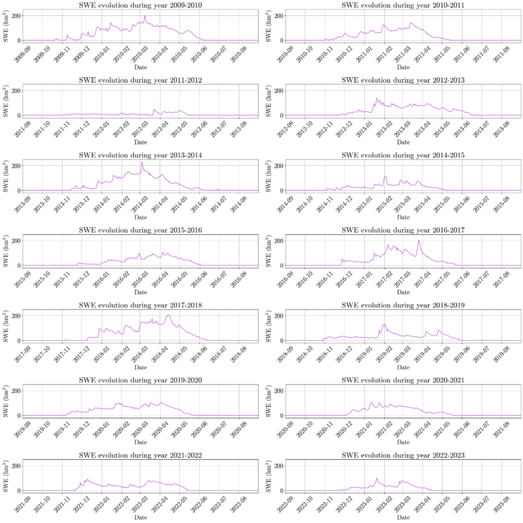
Figure 6: SWE time evolution for all years from 2009 to 2023.
3.2. Long term predictions
The objective is to predict the amount of water that is stored in the form of snow that will eventually reach the reservoir specifically for the snowmelt season. The snowmelt season can be defined as the period in which the thick layer of snowpack at the highest peaks of the region begins to continuously melt until only a minimal amount of permanent snow remains. This thawing process usually begins during early spring and ends later at the end of that same season, sometimes extending into the summer. To determine the start and end date of it, we can make use of the SWE curves that we computed in Section 2.3. The start would correspond to the time when a SWE maximum is observed, followed by a practically monotonous descent that eventually reaches a barely null SWE value, which would determine its end. Then, the SWE volume that reaches the reservoir throughout the snowmelt season will be the initial amount reported at the maximum in the date of start.
With respect to predictions in the long term about the amount of water arriving at the reservoir, the calculation of the SWE curves along with the data collected by the rain gauges and the reservoir input flow allow us to estimate what are known as the “runoff coefficients” of rain and snow, during the snowmelt season. For a given year, the amount of water VSnowmelt that will reach the reservoir during the snowmelt season can be computed as seen in Equation 3:


where VRainfall is the amount of rainwater that falls throughout the snowmelt season, VSnow is the SWE snowmelt volume that we described and obtained earlier, and CR and Cs are the runoff coefficients of rain and snow respectively. These coefficients represent the fact that not all the runoff water that enters and flows through the basin eventually reaches the reservoir. Because of this, they are confined to the range of [0,1].
To compute the received water volume at Barasona, we integrate in time the measured arriving flow from the start date of the snowmelt to its end date:


where ti is the start date of the snowmelt, tf is the end date of the snowmelt, and q(t) is the input flow at the Barasona reservoir.
For the rainfall, a similar procedure can be used integrating the average measured rainfall at the whole basin:

where now p(t) represents the rainfall, and A is the total area of the basin.
With these equations, now we have a triad of values for VSnowmelt, VRainfall and and VSnow for every year. To be able to extract from this data the values of the runoff coefficients, we assume that these values are constant during time or, at least, that they vary slowly enough in time so that our 14 years of calibration share the same coefficients. With this assumption, a simple least squares fit yields the value of the two parameters. The fitting will use all data points available (one per year) to determine the value of the coefficients CR and Cs presented in Equation 3.
3.3. Short term predictions
For the short term predictions we have relied on the LSTM model we introduced in Section 1. Recurrent neural networks (RNN) are a type of neural network where the hidden information processed by a neuron is able to flow back to a previous layer, allowing cycles between neurons (Goodfellow et al., 2016). This is contrary to what happens on a regular feed-forward neural network, where information transmission is unidirectional: from the input layer to the hidden layers, and eventually to the output neurons. RNNs are specialized in dealing with sequential data and can be especially useful when processing time series.
The structure of the most basic type of RNN is presented in Equations 6 and 7. In this RNN, the output of the hidden layer h(t) at a given time step is used as an input for the next step. x(t) would be the input sequence, and f is a function that represents the application of the weights (w and U) and the activation function as seen in Equation 7.



In this kind of RNN, h, also known as the “hidden state”, represents a compilation of the previous information seen by the neuron. However, a known issue of this type of RNN is the “vanishing gradient problem”, that hinders the prediction capabilities of the network by slowing down the learning process and causing the network to miss the long-term dependencies.
In Figure 7 we can see the basic diagram for a LSTM cell. The LSTM cell depends on the input x(t) and the hidden state from the previous timestep h(t-1). However, this model introduces a new state with respect to regular RNNs known as the cell state c(t). This variable is key to the capability of the cell to remember long term dependencies. In the LSTM cells, the hidden state contains the information from the previous timestep, and so the cell state represents the memory of the network. Using the different elements present in the cell, the cell state selectively stores, forgets, and outputs information, allowing the system to model complex patterns.

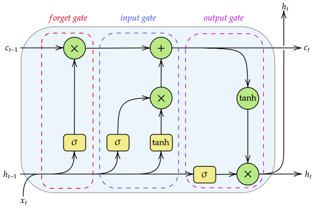
Figure 7: Block diagram for the LSTM cell.
The equations that make up the whole structure are the following:






where W and U represent the different weights of the layers inside each of the gates, b are the corresponding biases, and and tanh () represent a sigmoid and hyperbolic tangent operation respectively. The introduction of all these gates is what allows the LSTM cell to decide which information is stored from the last timestep, and which one is discarded, allowing long-term dependencies to be taken into account.
An important parameter of the LSTM cell is what is known as the number of units, or the “hidden size”. It corresponds to the dimensionality of the hidden state h(t), and can also be understood as the number of neurons used for this hidden state that are in every subgate. It is not straight-forward to know what this number of units should be, so it needs to be calibrated before fitting the definitive model.
Regarding the architecture of the model, our neural network will have an initial input layer, followed by a single LSTM, that leads to a final output layer. In the following lines, the loss function that we will use is the Mean Squared Error (MSE), as defined in Equation 13:


where n is the number of samples, yi is the actual value that we are trying to predict and is the prediction of our model. For the backpropagation we will use Adam, which is a stochastic gradient descent optimization algorithm based on adaptive estimates of lower-order moments (Kingma & Ba, 2014). All variables are also scaled to the range of [0,1] using min-max normalization (see Equation 14), which significantly increases prediction accuracy.

To tune the hyper-parameters of the neural network, we use a “time series split cross validation method”. In this validation technique, a small subset of the dataset starting from the earliest sample available is initially selected. This subset is divided into two sections: one for training, and another one for validating. Once this validation is done, the resulting validation loss is stored, and the size of the initial data subset is increased, taking more values closer to the latest sample available. This is repeated until the whole validation dataset has been covered. The average loss of all iterations is then taken as reference for comparing different network designs.
4. Results and Discussion
4.1. Long-term predictions
In Table 1, the calculated start and end date of the snowmelt season are displayed, along with the initial SWE volume. Notice how the dates differ from year to year, as well as the initial volume. The average start date computed finding the SWE maxima is the 23rd of March, with 16 days of standard deviation. The observed value of the initial volume presents large variability, since it completely depends on the amount of snow fallen during the previous winter, and so it is logically lower in years where the basin suffered from drought episodes, like in 2011-2012 (Linés et al., 2017). Overall, the average initial volume is of 120.27 hm3, and presents a standard deviation of 58.15 hm3. Lastly, the average end date is the 26th of May with 15 days standard deviation.
Table 1: Start date and end date for the snowmelt season for each year (day/month), along with the volume at the beginning of it.
| Hydrological Year | Start date | End date | Initial volume [hm3] |
| 2009-2010 | 18/3 | 9/6 | 199.31 |
| 2010-2011 | 9/3 | 15/5 | 142.66 |
| 2011-2012 | 26/3 | 24/5 | 48.82 |
| 2012-2013 | 9/4 | 16/6 | 93.76 |
| 2013-2014 | 30/3 | 7/6 | 228.77 |
| 2014-2015 | 26/3 | 7/5 | 73.90 |
| 2015-2016 | 12/4 | 4/6 | 107.55 |
| 2016-2017 | 6/4 | 24/5 | 184.39 |
| 2017-2018 | 15/4 | 15/6 | 206.72 |
| 2018-2019 | 14/4 | 30/5 | 80.01 |
| 2019-2020 | 1/4 | 29/5 | 101.05 |
| 2020-2021 | 24/3 | 19/5 | 60.04 |
| 2021-2022 | 13/3 | 16/5 | 79.60 |
| 2022-2023 | 7/3 | 19/4 | 77.27 |
The results of the fitting can be observed in Figure 8, where the predicted using the fitted coefficients and the yearly and values are plotted against the actual of that same year. The obtained value for the coefficients is CR=0.314 and Cs=0.320, meaning that only around a 30% of the overall water entering the basin eventually reaches the reservoir. As we can see, the results have a great accuracy, with a coefficient of determination of R2=0.90 and a RMSE of 31.63 hm3, computed as the root of the MSE. It is also worth noting that the coefficients calculated still hold even after a change in the total amount of water entering the basin (due to some years being drier than others). With these results we are able to provide an assessment of the SWE arriving at the Barasona reservoir, on which the CGR-CAyC had placed their interests to properly manage water distribution.

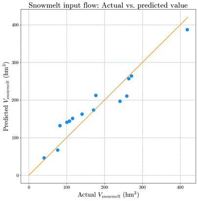
Figure 8: Actual vs. predicted value for the Barasona snowmelt input flow computed with the fitted runoff coefficients.
4.2. Short-term predictions
The objective is to predict, using the daily data presented in the previous sections, the Barasona reservoir input flow of the following day. The main model that we focus on uses the total SWE at the basin (also called simply “snow” during the rest of this section), the rainfall across the whole basin and the average temperature at the whole basin. We choose to use these as our input variables because, in a theoretical level, it should be enough data for the entering water flow to be calculable, since rain and snow are the main contributors to river flow and temperature provides seasonal information that the network might require. Using the time series split cross-validation technique we described in Section 3.2, we obtained that best performance was achieved when 20 LSTM units, a learning rate of 0.002 and 30 previous days of information were used.
Once this calibration is performed, we proceed to the production of the base model. We use a 70-30% training-test split of the whole dataset. The best network trained yielded a coefficient of determination of R2=0.691 and a RMSE of 9.35 m3/s. Figure 9 illustrates the dynamics of river flow, rain and snow along with our corresponding predictions during a randomly chosen two-year period. We can see how the predictions follow quite well the general trend of the flow variable. The effect of rain is very clear, causing a sharp increase in the reservoir flow, while the contribution of snow can mainly be noticed during thaw, when the streamflow experiences a small increase that lasts until summer. A plot of the actual values versus the predicted ones of the complete testing dataset can be seen in Figure 10 (marked as black circles). We see that most of the guesses are in the range of 0 to 0.2 (after normalization), and they concentrate around the ideal prediction line. However, the model has some difficulty when trying to guess larger values of the reservoir’s input flow. A possible reason for this might be the small number of values in this range, that makes it difficult for the model to be trained to guess them.

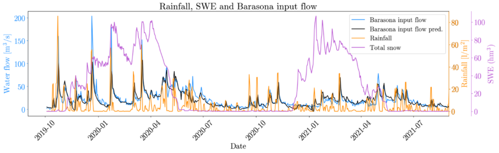
Figure 9. Dynamics of rainfall, snow, input flow at Barasona and its corresponding predictions from the base model between 2019 and 2021.

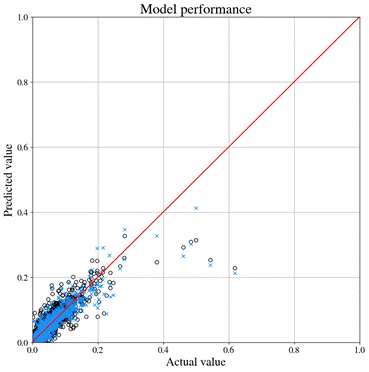
Figure 10: Actual value vs. predicted value of the Barasona input flow by the base model (black circles) and the model including the flow from previous days as an input (blue crosses). The ideal prediction is represented by a red line.
Another interesting property to analyze is the feature permutation importance. This technique allows us to assess the overall relevance that each of the variables has in the predictions of the model. To compute it, the fitted model is fed with the same testing dataset, but with one of the input variables randomly shuffled. This renders the variable useless for prediction purposes and causes an increase in the loss function that the model attempts to minimize. The larger this loss increase is, the more important a variable is for the predictions. We repeat this process 5 times for each variable, to ensure that the outcome is not a product of coincidence. The MSE of the normalized base model is 0.0008. The results of this analysis show that the most important feature of the model is rain, with an increased MSE of 0.0032. Snow and temperature cause each a similar loss increment, but only up to 0.0012. This might be explained by the fact that rainfall always represents a larger fraction of the water contribution to the reservoir’s lake when compared to snow, that only contributes during thaw.
A very logical change that could be introduced to the current model would be to include the past information of the Barasona input flow as an extra input to the model. Indeed, if the network can infer the flow from the temperature, rain and snow data from the previous days, then it might also be able to extract information from the previous days measured input. The resulting performance of the best fitted model including such variable is displayed in Figure 9 (blue crosses). Comparing with the previous performance at Figure 10, one notices that the sample values’ distribution is narrower around the ideal prediction line, meaning that the prediction improves when including this new variable. Notice however that days of large incoming flow are still not accurately guessed, with some predicted points being closer to their actual value, while other being further away. Despite this, there is an overall increment in accuracy when including this variable, as the increased and reduced RMSE of 7.88 m3/s values demonstrate. A reason for this could be that the Barasona input flow time series has a small but significant auto-regressive component, that the model can detect and subsequently learn to estimate the flow of the next day.
With respect to the feature permutation importance of the new model, we obtain that the flow variable has become the most relevant variable for the model to keep the loss to a minimum. If the baseline MSE of the new model is 0.00057, shuffling the input flow increases it to 0.0022. The next most important variable is rain, which still retains some importance, with an increased loss of 0.0016. But the importance given to the flow has come at the expense of the importance of the snow and temperature, which are now very low, increasing the MSE to around 0.0006 only. This is a sign that the input flow variable shares information that the model previously had found in the SWE and temperature variables. A physical explanation for this could be the fact that snow’s water contribution mostly takes place during thaw, around spring. This period is always followed by a slow increment of the amount of water arriving at the reservoir that lasts until a few weeks have passed after the basin runs out of snow, as we observed back in Figure 9. Seeing that this melting contribution varies so slowly and remains stable through the snowmelt, and looking at the feature importance difference between the two versions of the model, we conclude that providing the flow from the previous days already gives the model the snow contribution that was previously extracted from the SWE and the temperature. Along with this we also must take into account the mathematical correlation of short-time dependencies for the flow signal. In summary, it seems that snow and temperature are not too important to predict the input flow of the reservoir in the short term, as long as the flow from the previous days is provided.
We can compare our results with those from similar studies in the literature. Palazón and Navas (2016) applied the SWAT model to the Barasona reservoir basin to evaluate the influence of different climatic characterizations in river discharge at a monthly scale. The predicted river flow between 1994 and 1996 that they obtained at Graus, located very close to the reservoir, had a RMSE of 10.5 m3/s, that decreased to 7.7 m3/s when creating a synthetic weather station for an intermediate point of the Ésera headwater. Both results lie in a similar range to ours. Regarding the application of river flow forecasting neural network models in other basins, we can highlight the results of Firat (2008), which used two different neural network models (feed-forward neural network and generalized regression neural network) to predict the streamflow of the Cine River using precipitation data and the flow from previous days. They obtained, for their best neural network model, a coefficient of determination of R2=0.738, which is also quite similar to ours.
5. Conclusions
In this study, we have successfully improved the computation of the snowmelt volume available for the Barasona reservoir for the past 14 years, utilizing data from 15 different in-situ sensors and from three remote sensing sources: MODIS, Sentinel 2 and Landsat 8. The data obtained has proven to be useful to perform predictions both in the short and long term.
With respect to predictions in the long-term, we have been able to obtain the snowmelt volume available at the start of the snowmelt season. This volume largely fluctuates throughout the years, with an average of 120.27 hm3 and a standard deviation of 58.15hm3. For the past year, our calculations place this SWE at 77.27 hm3. We also have been able to estimate the average start and end date for the snowmelt season using the SWE curves, around March 23 and May 26, with around 2 weeks of standard deviation for both. Combining all this information with the rainfall and the input flow during the same time period, we have been able to estimate the basin runoff coefficients of snow and rain as CR=0.314 and Cs=0.320, using a least squares fitting of R2=0.90 , under the assumption that they stay constant in our 14 years of data. With all this data and the methods described in our study, one can estimate the SWE that will reach the Barasona reservoir basin. This type of information is useful so that educated decisions can be made in regard to the management of the water supply to the corresponding agricultural holdings, especially in situations of drought, where water is scarce. Snow, as opposed to rain, is an asset whose yearly contribution is mostly already fixed by the beginning of snowmelt, so it provides a guaranteed minimal water volume that will arrive at the basin that is not dependent on future weather conditions, which is key to properly administer irrigation water supply.
We also trained a recurrent neural network model based on the Long-Short Term Memory cell that predicted the input flow of water for the Barasona reservoir in the short-term, with maximum accuracy achieved when forecasting the flow of the following day, with R2=0.691. The inputs for the base model that we presented included the average rainfall of the basin, the total SWE volume observed, and the average temperature of the basin. Rain and snow represent the largest contributions of water that the basin could receive during a hydrological year, while temperature provides information concerning the season of the year. The model predicts adequately the flow in most days, but underpredicts it when it increases. This might be due to the lack of data available in that value range. Other reasons for this phenomenon but also for other minor inaccuracies could be the complexity of hydrological processes of an admitted smaller scale yet of some relevance, such as water evaporation, sun irradiance, underground processes and soil infiltration, the dense vegetation of the region, and human intervention. The region we deal with presents extreme temperatures changes in some sectors, and part of the water of the Ésera river is also diverted into a karst system. The influence of these factors is left for the model to estimate through its training from the three variables inputted, but it could be beneficial for it to be fed with some data that took some of these processes into account, which could drive the model’s accuracy up. Finally, there could be some small errors in the inputs we provided, that confuse the model and bring the accuracy down.
Including the information of the Barasona flow from the previous days as an input into the model increases the accuracy up to R2=0.781. This increase in accuracy represented a decrease in the importance for the model predictions of the snow and temperature, indicating that they are not significant for short-term forecasting on the condition that the input flow from previous days is provided. Situations where this might not be possible are uncommon but could include a temporal malfunctioning of the river gauge, or simply predictions applied to watercourses where the flow is not being monitored, although for the model to be trained, some sort of flow measurement campaign during some period would at least be required.
The results from our study open several research avenues. First, applying the methodology to another basin would help to confirm or rebut the validity of the methods proposed in this work. Regarding the temporal interpolation gap filling, it would be interesting to consider not only temporal data, but also geographical information of the empty pixels and their surroundings and use this to infer the pixel’s snow cover percentage. For the computation of the basin temperature, precipitation and snow volume, our methods are as limited as the geographical distribution of the instruments is. As it has been shown, the basin overall would benefit from the installation of more weather stations, especially at the higher altitudes of it. Nevertheless, it would be of great interest to try other interpolating techniques and compare the results and performance. Finally, for the neural network model, a possible improvement could be a redefinition of the loss function, giving more weight to days with large input flow, and see if the model improves the corresponding forecasts. There are also other architectural options still left to explore. For example, since the data we produced takes the form of two-dimensional rasters, a potential future line of work could be to adapt the LSTM model to use these directly as an input, perhaps by introducing convolutional layers to the neural network.
Autor Contributions
L. López: Conceptualization, data curation, formal analysis, investigation, methodology, software, validation, visualization, writing original draft. M. J. Escorihuela: Conceptualization, formal analysis, investigation,methodology, project administration, resources, supervision, writing review and editing. All authors have read and agreed to the published version of the manuscript.
Declaration of Competing Interest
The authors declare that they have no known competing financial interests or personal relationships that could have appeared to influence the work reported in this paper.
Data availability
Data will be made available on request.
Acknowledgments
We are grateful to the CGR-CAyC for their support with this research.
References
Arnold, J. G., R. Srinivasan, R. S. Muttiah, and J. R. Williams. 1998. Large-area hydrologic modeling and assessment: Part I. Model development. J. American Water Resources Assoc. 34(1): 73-89. https://doi.org/10.1111/j.1752-1688.1998.tb05961.x
CAyC, n.d. Zona Regable https://www.cayc.es/index.php/es/entidad/zona-regable (accessed December 11th, 2024).
CHE, n.d. Canal de Aragón y Cataluña. https://www.chebro.es/canal-de-aragon-y-catalu%C3%B1a (accessed December 11th, 2024).
CHE, 2002a. Estudio de la calidad ecológica integral de los tramos fluviales más importantes del río Cinca – río Ésera – Informe de Síntesis. https://www.chebro.es/documents/20121/66562/06eseraSintesis.pdf/87a6faaa-5348-245b-731c-23dad772a429
CHE, 2002b. Estudio de la calidad ecológica integral de los tramos fluviales más importantes del río Cinca – río Isábena – Informe de Síntesis. https://www.chebro.es/documents/20121/66562/10isabenaSintesis.pdf/74a82058-ec74-692e-2a8c-b8cc0a0e287c
Dozier, J., 1989. Spectral signature of alpine snow cover from the Landsat Thematic Mapper, Remote Sens. Environ., 28, 9–22 https://doi.org/10.1016/0034-4257(89)90101-6
ESA, n.d. Introducing Sentinel 2. https://www.esa.int/Applications/Observing_the_Earth/Copernicus/Sentinel-2/Introducing_Sentinel-2 (accessed December 11th, 2024).
ESRI, n.d. Thiessen Polygons. https://support.esri.com/en-us/gis-dictionary/thiessen-polygon (accessed December 11th, 2024).
Fassnacht, S. R., Heun, C. M., Lopez-Moreno, J.-I., Latron, J. , 2010. Variability of Snow Density Measurements in the Rio Ésera Valley. Colorado State University. https://doi.org/10.18172/cig.1227
Firat, M. Comparison of Artificial Intelligence Techniques for river flow forecasting. Hydrol. Earth Syst. Sci., 12, 123–139, 2008 www.hydrol-earth-syst-sci.net/12/123/2008/ (accessed February 22nd, 2025)
Gascoin, S., Grizonnet, M., Bouchet, M., Salgues, G., and Hagolle, O., 2019. Theia Snow collection: high-resolution operational snow cover maps from Sentinel-2 and Landsat-8 data, Earth Syst. Sci. Data, 11, 493–514. https://doi.org/10.5194/essd-11-493-2019
Gazol, A., Sangüesa-Barreda, G., Camarero, J. J., 2020. Forecasting Forest Vulnerability to Drought in Pyrenean Silver Fir Forests Showing Dieback, Front. For. Glob. Change, Sec. Forest Hydrology, Volume 3. https://doi.org/10.3389/ffgc.2020.00036
GDAL, n.d. GDAL Documentation. https://gdal.org/index.html (accessed December 11th, 2024).
Gers, F.A. , Schmidhuber, J., Cummins, F., 2000. Learning to Forget: Continual Prediction with LSTM. Neural Computation 12 (10): 2451–2471. https://doi.org/10.1162/089976600300015015
Goodfellow, I., Bengio, Y., Courville, A., 2016. Deep Learning, The MIT Press, 1st Edition. ISBN: 978-0262035613
HEC-HMS, n.d. Snow Properties. https://www.hec.usace.army.mil/confluence/hmsdocs/hmstrm/snow-accumulation-and-melt/snow-properties (accessed December 11th, 2024).
Hochreiter, S., Schmidhuber, J., 1997. Long Short-Term Memory, Neural Computation, 9 (8): 1735-1780. https://doi.org/10.1162/neco.1997.9.8.1735
Jacobson, M. Z., 2005. Fundamentals of Atmospheric Modeling (2nd ed.). Cambridge University Press. ISBN 978-0-521-83970-9.
Kingma, D., Ba, J., 2015. Adam: A Method for Stochastic Optimization, 3rd International Conference for Learning Representations, San Diego. https://doi.org/10.48550/arXiv.1412.6980
Landsat, n.d. Landsat Science. https://landsat.gsfc.nasa.gov/ (accessed December 11th, 2024).
Linés, C., Iglesias, A., Garrote, L., Sotés, V., Werner, M. , 2018. Do users benefit from additional information in support of operational drought management decisions in the Ebro basin?, Hydrology and Earth System Sciences. https://doi.org/10.5194/hess-22-5901-2018
Linés, C., Werner, M., and Bastiaanssen, W., 2017. The predictability of reported drought events and impacts in the Ebro Basin using six different remote sensing data sets, Hydrol. Earth Syst. Sci., 21, 4747–4765. https://doi.org/10.5194/hess-21-4747-2017
MODIS, n.d. About MODIS. https://modis.gsfc.nasa.gov/about/ (accessed March 3rd, 2024).
Muskett, R. R., 2012. Remote Sensing, Model-Derived and Ground Measurements of Snow Water Equivalent and Snow Density in Alaska. International Journal of Geosciences, 3, 1127-1136. http://dx.doi.org/10.4236/ijg.2012.35114
NASA, n.d. MODIS Snow Cover. https://modis.gsfc.nasa.gov/data/dataprod/mod10.php (accessed December 11th, 2024).
Palazón, L., Navas, A., 2016. Case Study: Effect of Climatic Characterization on River Discharge in an Alpine-Prealpine Catchment of the Spanish Pyrenees Using the SWAT Model, Water 2016, 8, 41
Patterson, W. S. B., 1994. The Physics of Glaciers. 3rd Edition, Oxford. ISBN 0-08037945 1
Reynaud, A., 2008. Economic impacts of drought on agriculture, INRAE Sciences Sociales, Institut national de recherche pour l’agriculture, l’alimentation et l’environnement (INRAE), Departement Sciences Sociales, Agriculture et Alimentation, Espace et Environnement (SAE2), vol. 2008, pages 1-6, September. https://doi.org/10.22004/ag.econ.155277
Theia, n.d. Value-Adding Products and Algorithms for Land Surfaces. https://www.theia-land.fr/en/homepage-en/ (accessed December 11th, 2024).
Ulbrich, U., May, W., Li, L., Lionello P., Pinto, J.G., Somot, S., Chapter 8 The Mediterranean climate change under global warming, Developments in Earth and Environmental Sciences, Elsevier, Volume 4, 2006, Pages 399-415, https://doi.org/10.1016/S1571-9197(06)80011-X
USGS, n.d. Earth Explorer, https://earthexplorer.usgs.gov/ (accessed December 11th, 2024).
Veiga, V.B., Hassan, Q.K., He, J., 2014. Development of flow forecasting models in the Bow River at Calgary, Alberta, Canada. Water 2015, 7(1), 99-115; https://doi.org/10.3390/w7010099
Zhao, Hongling, Hongyan Li, Yunqing Xuan, Changhai Li, and Heshan Ni. 2022. Improvement of the SWAT Model for Snowmelt Runoff Simulation in Seasonal Snowmelt Area Using Remote Sensing Data. Remote Sensing 14, no. 22: 5823. https://doi.org/10.3390/rs14225823
Žiga M., Verburg, P. H., 2017. Adaptation of land management in the Mediterranean under scenarios of irrigation water use and availability. Mitigation and Adaptation Strategies for Global Change, 23, pages 821–837, (2018) https://doi.org/10.1007/s11027-017-9761-0
Publisher’s Note
The statements, opinions and data contained in all publications are solely those of the individual author(s) and contributor(s) and not of Recent Advances S.L. and/or the editor(s). Recent Advances S.L. and/or the editor(s) disclaim responsability for any injury to people or property resulting from any ideas, methods, instructions or products referred to in the content.