


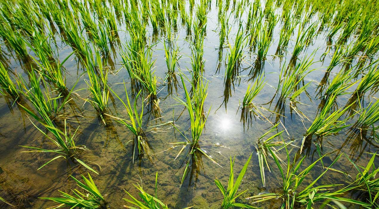
Mapping rice and wheat crops in Egypt’s Nile Delta using Sentinel-2 from 2018 to 2022
César J. Guerrero Benavent
1*,Belen Franch

1,2, 
Guillem Sòria
1, Italo Moletto-Lobos
1, Javier Tarín
1, Katarzyna Cyran
1- Global Change Unit, Parc Cientıfic, University of Valencia, Paterna, 4498, Valencia, Spain.
- Dept of Geographical Sciencies, Univesity of Maryland, College Park MD, 20742, United States.
* Author to whom correspondence should be addressed.


Abstract
Mapping crop types is vital for quantifying cultivated areas and supports agricultural statistics, land use analysis, and crop yield predictions. This study focuses on creating accurate rice and wheat crop type masks in Egypt’s Nile Delta, specifically in the Gharbia governorate, from 2018 to 2022, in the context of EO Africa initiative. Crop type maps for both, summer and winter seasons were developed using a Random Forest method. A set of ground truth points for each year, majorly of rice and wheat but also a few of onion, maize, clover, citrus and grape crops were filtered and completed analytically to be used as training and test data. To face imbalance, Synthetic Minority Oversampling Technique (SMOTE) method was also applied, generating synthetic data of the non-interest crops. The masking method consisted in extracting the spectral information of these points for all the selected cloud-masked Sentinel-2 images of the season. This information was stacked, obtaining several features equal to the number of spectral bands per number of images of the season considered. This set was optimized through a PCA analysis applied over the spectral bands, reducing the number of features to the 25-30 first components. For each image, also different vegetation and water indices (NDVI, DVI, SAVI, NDWI, AWEI, EVI) were computed and stacked to the previous set to conform the final features space, reducing dimensionality and showing the best results compared with the application of PCA to the complet set (bands and indices). This process was applied to each season, obtaining an accuracy between 0.85 and 0.95 and consistent commission and omission errors, meaning balanced estimations. From the final classification map, rice and wheat classes were extracted, obtaining preliminary masks. Finally, isolated pixels were removed, and possible detection holes were covered with the use of morphology techniques (opening and closing), obtaining final operational masks.Keywords
Crop type, Machine Learning, Nile Delta, Sentinel-2, Random Forest1. Introduction
According to the 2023 African Regional Overview of Food Security and Nutrition [1] developed by FAO (Food and Agriculture Organization of the United Nations), AU (African Union), ECA (United Nations Economic Commission for Africa) and the WFP (World Food Program), Africa is facing a severe food crisis. In some regions, most people do not have access to a basic healthy diet, which cost increases progressively. Despite that agriculture is the most important sector, [2] reports that Africa has the 60 percent of the world’s uncultivated arable land. In fact, the underdeveloped infrastructure in some countries makes the agricultural production of small farmers essential to provide food to the population. It is also worth highlighting here the negative impact in agricultural production of the rising temperatures due to climate change. Given this evidence of a critical panorama for food security, there is a global need to put efforts into achieving more sustainable and optimized food and agricultural management that meets the needs of the population.
Egypt is an example of the situation described above, where approx- imately 11.3% of the country’s gross domestic product comes from the agricultural sector [3]. Given that only 4% of the land in Egypt is arable and mainly located at Nile Delta [4], the agricultural activity in this area is maximum and is mainly represented by small landholdings that generally do not meet international standards. However, despite the wealth of Nile’s Delta land resulted by its fertile soil and abundant water supply, a study of NASA Earth Observatory (EO) performed in 2021 [5] claimed that the farmland of this region shows a decreasing trend mainly caused by urbanization, which could cause severe food security problems in Egypt.
With a clear necessity of increasing and improving the quality of food production while suitable area for agriculture is reduced and the amount of population increases, accurate and timely information on crop agriculture variables, as for example crop yields or phenological development stages, can play a crucial role. Remote sensing can then be used to obtain periodically and in a spatially continuous way some of this information, monitoring the crop growth from early stages to the harvest and helping farmers in decision making. It has to be said that from the remote sensing perspective, Africa is also one of the most challenging locations, since as said before, agriculture is mainly represented by small farms, which can be challenging to monitor because of the spatial resolution limitations of some satellite products.
The EO Africa initiative [6] launched by European Space Agency (ESA) aims to harness the potential of the Earth observation technologies to support sustainable development and environmental management across Africa. This program focuses on capacity building, fostering the use of satellite data for informed decision-making in critical areas such as agriculture, water resources, climate change adaptation, or disaster risk management. Within the frame of this initiative, and establishing a collaboration between the University of Tanta (Gharbia, Egypt) and the University of Valencia (Valencia, Spain), a project focused on the use of high spatial and temporal resolution data for monitoring wheat and rice crop agronomic variables for smallholder agriculture in the Nile Delta was conceived. The main goal of the project is the development of rice and wheat yield models [7]. These models are build over the Gharbia governorate, which is one of the most significant regions concerning agricultural production within the Nile Delta, and it is a critical area for food security in the country.


Figure 1: Location map of Gharbia governorate (Egypt).
This paper exposes a complete workflow for the generation of seasonal crop type masks for rice and wheat crops from year 2018 to 2022. These masks are a necessary prerequisite for the application of yield models, since they facilitate the isolated study of the target crops, reducing errors and optimizing the model employed. For this purpose, an analytical process is presented to generate ground truth data, dealing with a limited initial data set that is refined and increased. For this refined data, time series of Sentinel-2 images are retrieved to extract all the available spectral information together with a set of vegetation and water indices, which are used to feed a classification model based on a Random Forest algorithm. Finally, rice and wheat masks are created by extracting these crops from the seasonal crop type maps.
2. Study area and materials
2.1. Study area
This work is carried out over the Gharbia Governorate, Egypt, a region close to the center of Nile Delta (Figure 1). This region has a dry climate, registering normally less than 20 mm of precipitation per month. December and January are the coldest months with average temperatures going from 20 to 25◦C; while between April and October a hot season is found, achieving average maximum temperatures of 36◦C in the warmest scenarios [8]. In the territory of Gharbia, up to fifteen types of crops can be found typically grouped in small, irregularly shaped plots; additionally, crop rotation is practiced in this area. Cereal crops such as rice, maize, wheat or barley predominate; however, the region of Gharbia also contains fields dedicated to fruit crops, palm trees, clover crops, vegetables, etc.
The Nile Delta represents the 80% of the total rice production in Egypt, specifically, Gharbia governorate has the 14% of this production [9] turning this crop into an important staple food in the region. Rice is a summer crop generally produced between May and October. It is irrigated through continuous flooding and then is dried just before the harvesting stage. This technique is really water consuming and has lead in the last years to an intensive research with the goal to develop more sustainable ways to proceed [10].
The Nile Delta also contributes considerably to the wheat production. Approximately the 60 − 65% of the Egypt’s wheat is produced in the Nile Delta. Particularly, Gharbia is responsible of the 5% of this production [9]. Wheat is a staple cereal known for its versatility and adaptability to various climates, especially in temperate regions. It is usually produced in winter season, from October to April. The cultivation involves several steps, like soil preparation, where the soil is plowed and leveled to generate a seedbed; irrigation, enhanced by the water supplies of Nile Delta; and generally, fertilization and pest control.
2.2. Materials
2.2.1. Remote sensing data
To perform in-season classification, time series of Sentinel-2 images from 2018 to 2022 were used, which counts with a total of 13 spectral bands, 4 in the visible range (the aerosol band with 60 m resolution and the RGB bands with 10 m resolution), 6 in the NIR range (with 20 m and 10 m resolution except the water vapor band with 60 m resolution), and 3 bands in the SWIR range of the spectrum (all of them with 20 m resolution except the cirrus band with 60 m resolution). Level 1 C data was downloaded and atmospherically corrected using LaSRC (Land Surface Reflectance Code) by Vermote et al. [11], the atmospheric correction algorithm used in the generation of surface reflectance products of Earth Observation missions such as Landsat-8 and Landsat-9. LaSRC was selected due to its good performance in correcting aerosol effects, which have a strong impact in the visible and Near-Infrared bands of Sentinel-2 as shown by the Atmospheric Correction Intercomparison eXercies (ACIX) [12].
To cover the region of Gharbia, tiles 36RTV and 36RUV were needed (Figure 2); therefore, these two tiles were processed, merged and cropped downscaling all bands to 10 m resolution to obtain single and lighter multiband images to optimize and reduce the computational cost of the subsequent described processes. All these images were cloud masked with the s2cloudless algorithm [13] using an input treshold of 0.2 . Furthermore, cloud shadows were taken into account using the cloud mask projection available in Google Earth Engine [14]; in this case, considering a 2 km shadow extension and a NIR treshold of 0.15. It is worth saying that Gharbia is located in the overlap region of two Sentinel-2 orbits (Figure 2), obtaining images every 2-3 days, despite the typical revisit time of 5 days provided by Sentinel-2A and Sentinel-2B together.
2.2.2. In situ ground truth data
A set of in situ ground truth data was provided by the Tanta’s University partner under the frame of ESA EO Africa project. This dataset provided the historical evolution of a set of geolocated plots within the Gharbia governorate, indicating their geographical coordinates and the crop type, and distinguishing between winter and summer seasons (accounting for crop rotation). The database was majorly composed by rice and wheat plots, but it also indicated some citrus (and some other fruit trees), grape, clover, maize and onion plots. Particularly, 214 locations of wheat and rice fields were registered along the seasons 2016-2022. All this data was reorganized per years focusing on the period 2018 to 2022. Based on this dataset, the proposed classification maps were intended to contain 5 classes, with differences depending on the season: for the summer season maps, classes were rice, MOC (mainly maize), grape, citrus and water-urban; complementary, for the winter season maps, classes were wheat, MOC (mainly clover and onion), grape, citrus and water-urban.
2.2.3. Crop calendars
For the purpose of this study, the use of crop calendars was also crucial. With them, main phenological stages Start Of Season (SOS) and End Of Season (EOS) of different crops can be identified in time particularly for each year. Calendars used here are developed in [15]. In this referenced work, Sen2like [27] and PlanetScope Normalized Difference Vegetation Index (NDVI) [28] series are employed to estimate the start of season and the end of season at regional level for the Gharbia governorate. Table 1,2,3 and 4 show the most important calendars for the aim of this work.
For a better interpretation of these calendars, Figure 3 was generated to study the overlaps between summer and winter crops. The identification of these overlaps will be key for the generation of new ground truth data through visual analysis, which is described for each crop in more detail in the following section of this text. The error in the determination of the SOS and EOS dates of the model presented in [15] are of primary importance, since the SOS and EOS can vary considerably across the region due to different agricultural practices or different external conditions.


Figure 2: Tile grid (red squares) and relative orbits (black lines) of Sentinel-2A and 2B (a) and tiles 36RTV and 36RUV used to cover Gharbia region (b).
Table 1: Rice yearly phenological calendar.
| RICE | SOS | EOS |
| 2018 | 31 May ± 17 days | 19 Sep ± 13 days |
| 2019 | 6 Jun ± 18 days | 22 Sep ± 17 days |
| 2020 | 2 Jun ± 16 days | 2 Oct ± 15 days |
| 2021 | 2 Jun ± 19 days | 22 Sep ± 16 days |
| 2022 | 19 May ± 4 days | 6 Oct ± 4 days |
Table 2: Maize yearly phenological calendar.
| MAIZE | SOS | EOS |
| 2018 | 27 May ± 13 days | 14 Sep ± 13 days |
| 2019 | 6 Jun ± 17 days | 23 Sep ± 15 days |
| 2020 | 29 May ± 18 days | 18 Sep ± 15 days |
| 2021 | 4 Jun ± 15 days | 26 Sep ± 12 days |
| 2022 | 10 Jun ± 11 days | 2 Oct ± 8 days |
Table 3: Wheat yearly phenological calendar. EOS dates refer to the next year.
| CLOVER | SOS | EOS |
| 2018 | 4 Nov ± 6 days | 11 Apr ± 8 days |
| 2019 | 25 Oct ± 7 days | 12 Apr ± 9 days |
| 2020 | 5 Nov ± 15 days | 12 Apr ± 7 days |
| 2021 | 9 Nov ± 11 days | 17 Apr ± 8 days |
| 2022 | 10 Nov ± 10 days | 21 Apr ± 6 days |
Table 4: Clover yearly phenological calendar. EOS dates refer to the next year.
| CLOVER | SOS | EOS |
| 2018 | 15 Oct ± 6 days | 4 May ± 14 days |
| 2019 | 4 Oct ± 7 days | 8 May ± 17 days |
| 2020 | 12 Oct ± 9 days | 11 May ± 18 days |
| 2021 | 10 Oct ± 5 days | 10 May ± 17 days |
| 2022 | 30 Oct ± 7 days | 16 May ± 16 days |
3. Methodology
3.1. In situ ground truth data curation
The ground truth data obtained from Tanta University was first subjected to a quality analysis. First steps consisted in the digitalization of the points and the drawing of the parcel polygons delimiting the fields based on last available Google Maps imagery. After that, some of the points were removed from the set due to the poor precission observed in the geolocation by comparing with very high resolution satellite imagery.


Figure 3: Graphic representation of crop calendars. The figure on the top, shows rice and maize crop calendars (summer crops). The two figures below represent the crop calendars for wheat and clover (winter crops), note the change of the year in the y axis. Black whiskers at the end of the bars represent the error in the determination of SOS and EOS dates.
Considering also the spatial resolution of 10 × 10 meters of Sentinel-2 multispectral images generated for this study, fields with dimensions under this resolution were removed. Next, based on the parcel polygons, Sentinel- 2 surface reflectance data at field level was extracted, computing the average and standard deviation for each plot in each available acquisition during the season.
The NDVI index was calculated for each individual plot, since this index allows to distinguish the phenology of different crops. The results indicated that some parcels marked as cultivated showed no vegetation signature while others showed a different phenological evolution than the expected by the crop type indicated in the database. A restrictive filtering was performed in order to exclude from the study any parcel whose NDVI evolution did not follow the expected evolution of the tagged crop type, as the example showed in Figure 4 for wheat. After removing all these artifacts, the amount of points was considerably reduced. Table 5 shows the number of parcels for each crop (rice or wheat) within each year after the filtering. It is clear that the number of validated parcels was generally insufficient in most instances, creating a difficult context for the subsequent application of machine learning methods.
3.2. Generation of ground truth database
The lack of quality ground truth data is a really common challenge in remote sensing. Especially when applying Deep Learning techniques, the amount of data and how well it captures the heterogeneity of the area of interest, strongly conditions the transferability and generalisability of the subsequent developed models [16, 17]. The analysis described in section 3.1 lead to a poor database, which was not suitable for the development of machine learning methods, that generally need high volumes of reliable data to build robust models. The methodology proposed to address this issue is exposed next.


Figure 4: Filtration of parcels using NDVI series. Example for wheat season 2022. Date is indicated with the Day Of the Year (DOY)
Table 5: Results of the NDVI filtering applied to the initial ground truth data set. Each amount corresponds to rice and wheat parcels within the respective year.
| Year | Season | Amount of samples before filtering | Amount of samples after filtering |
| 2018 | Rice | 2 | 2 |
| Wheat | 65 | 16 | |
| 2019 | Rice | 55 | 45 |
| Wheat | 18 | 2 | |
| 2020 | Rice | 1 | 1 |
| Wheat | 62 | 17 | |
| 2021 | Rice | 60 | 36 |
| Wheat | 60 | 5 | |
| 2022 | Rice | 3 | 1 |
| Wheat | 45 | 9 |
To complement this limited data set, an exhaustive visual analysis was done with the goal of detecting several new samples of the crops for classification, especially of the main ones, rice and wheat. The proposed methodology for this analysis was based on the yearly identification of the harvesting (EOS) and planting (SOS) dates for each crop, which was done using the crop calendars introduced in the previous section of this text. The identification of harvested parcels within correct EOS dates was considered as a potential detected sample for the respective crop. However, an extra attention had to be paid for those crops with overlapping phenological stages, especially during the end of season, as it is the case for rice and maize. Note the importance of determination errors in crop calendars, as they enable the detection of these situations. For those crops, additional filtering was applied with the aim of discriminating rice crops against maize crops. The following subsections explain in detail the generation of the ground truth data for all the crops considered in this study.
3.2.1. Summer season: rice and maize.
During the summer season, mainly rice an maize crops are found. To increase the amount of rice ground truth points over the region of interest, crop calendars were used to identify SOS and EOS dates within the estimation error showed in Table 1 and 2. The principal objective was the detection of harvested fields during the EOS. However, these calendars showed a none negligible overlap between the harvesting period of rice and maize (Figure 3), which during this stage, and recalling the spatial resolution of Sentinel-2 images, could not be distinguished visually. During the SOS, rice fields are flooded and the reflectance signal coming from these crops is purely due to these shallow waters, since there is no vegetation contribution to the signal at this early stage of growth. Consequently, efforts to recognize rice crops were concentrated on the initial flooding stage.


Figure 5: Generation of the AWEI mask for the entire SOS (σ stands for the SOS error). AWEI images and flood masks were daily generated for each available Sentinel-2 scene and combined into a final flooded mask for the complete period.
For water detection, the AWEI (Automated Water Extraction Index) was employed. This index, was proposed by Feysa et al. [18] to address the problems presented by other commonly used water indices as the NDWI (Normalized Difference Water Index) [19] and the MNDWI (Modified Normalized Difference Water Index) [20] when separating water bodies from build-up areas or shadows respectively. The AWEI index is computed using a set of empirical coefficients determined based on reflectance patterns observed over pure pixels of different land covers. These coefficients were determined by identifying those that maximized the separability of water and non water surfaces, generally characterized by low reflectance in the NIR band [18]. AWEI index is calculated as follows:
AWEI = 4 · (GREEN − S WIR2) − (0.25 · NIR + 2.75 · S WIR1) (1)
taking positive values for open waters, zero or slightly negative for other water bodies or shallow water, and greater negative values for the non presence of water.
AWEI images for the SOS period of each year were generated. After an analysis of well-known examples of shallow waters in the scene (e.g. irrigation ditches), a threshold of -0.6 was established and pixels with AWEI values greater than this were considered as potential flooded plots. To account for the variability in the start of the flooding among the whole governorate, a unique mask was composed by the combination (union) of all AWEI daily masks composed for the SOS acquisitions within its determination error. This process is schematically described in Figure 5.
Figure 6 shows an example of the daily AWEI images generated during the process (a) and the respective AWEI > -0.6 mask. The AWEI mask developed for the complete SOS (Figure 6(c)) was then inverted and applied over the harvesting dates, acting as a window through which harvested parcels are selected. This new points satisfied the flooding condition and thus, were considered as rice plots. Figure 7 shows a schematic description of the previous process zoomed in a random area of Gharbia. The same steps described here were followed for the identification of maize plots; in this case, without the inversion of the AWEI SOS mask, in order to isolate areas that were not flooded during the start of the season.


Figure 6: Example of AWEI image (a), AWEI>-0.6 mask (b) and AWEI SOS mask (c) for the rice season of 2021.
3.2.2. Winter season: wheat and clover
The case for wheat is simpler than for rice. Despite that phenological calendars in Figure 3 show a clear similarity between clover and wheat harvesting stages, only 2021 shows a small overlap within the harvesting dates determination error. Based on this, and as exposed before, efforts where focused on identifying directly harvested parcels within the wheat EOS images. This process was done exhaustively for wheat, and complementary, for clover, using the corresponding dates in each case. Figure 8 shows an schematic overview for this first crop. Note that during early and middle EOS, the ripening stage of the wheat could be visually identified in some cases. This stage is characterized by the wheat kernels reaching maturity and losing chlorophyll, resulting in a yellowish coloration. This is different for clover crops, which during EOS, were observed to turn lighter green or even brownish color, but did not became as distinctly yellow as wheat.
3.2.3. Other crops, urban and water areas
In addition to the previously mentioned crops, Gharbia also contains areas dedicated to fruit trees (mainly citrus) and grapes. However, the number of ground truth points for these crops was limited and concentrated in small regions of the governorate. To address this, additional citrus points were identified through photo-interpretation using Google Maps imagery (Figure 9). This approach leveraged the fact that citrus crops have long growing cycles, meaning they remain consistent over extended periods. By using the initial ground truth points as a reference, similar parcels were identified in the last available aerial images of Google Maps and considered as ground truth data for this class with high confidence based on their stability over previous years. This technique was also tested with grape crops. However, due to the shorter growing period of grapes, this method occasionally introduced noise into the classification. As a result, the increase in grape parcels was not as notable.


Figure 7: Selection of rice ground truth data using the inverted AWEI SOS mask and the harvesting dates. Images show a randomly selected area as example before the EOS (top) and during the EOS (bottom). Black areas represent cloud masked regions.
The same technique was used for the creation of water and urban areas database. A set of points were selected homogeneously among the whole study area, including, cities, small buildings, roads, large water bodies (Nile Delta river) or small water bodies (mainly irrigation ditches). These areas are subsequently masked in the resulting crop type maps generated in this study.
3.3. Imbalanced learning SMOTE
By following the previously described workflow for generating ground truth data, the initial limited dataset was notably enhanced, particularly for the primary crops of interest: rice and wheat. Initially, the amount of points for these crops was already considerably higher than for citrus, maize, onion, clover and grape; and this disparity remained even after the generation of new data. This difference in the amount of samples among classes in the training dataset receives the name of imbalanced learning, and may introduce a clear bias towards the classes with greater representation.


Figure 8: Selection of wheat ground truth data using the harvesting dates. Images show a randomly selected area as example before the EOS (top), in the early EOS (middle) and in the late stages of the EOS (bottom). Black areas represent cloud masked regions.
SMOTE (Synthetic Minority Oversampling Technique) [21] is an algorithm that generates synthetic data based on real data examples of a given class. The purpose of this is to over-sample the minority classes till the amount of training data is equal to the majority class. The algorithm proceeds as follows: first, a real example of the minority class is taken together with its k nearest neighbors; second, a random selection among this neighbors is performed, depending on the amount of data that has to be generated (if the user wants to generate the double of the initial value of points, 1 of the k nearest neighbors is selected); next, the position vectors in feature space (i.e. the vector defining the points where each coordinate corresponds to each feature value of this point) from both the considered point and the neighbor, are computed and the difference between both is calculated; and finally, the differences between each coordinate is multiplied by a random number between 0 and 1 , and after that, these differences are summed to the considered real feature vector, generating a new one that represents a synthetic point.
3.4. Time series conformation, data retrieval and model construction
After accounting for the imbalanced training dataset, next step consisted in the retrieval of time series spectral data for each of the crops. These retrieval process started from the already merged and cropped images of the Gharbia region conformed with tiles 36RTV and 36RUV. Since the cloudless mask was applied, to avoid the consideration of images with larger masked regions that would generate data gaps, a filter of less than 15% of masked regions was applied. Table 6 shows the amount of images that result of the application of this filter for each year and season. Note that for rice season (summer season) the amount of images satisfying this condition is always greater. Because of this, another manual selection of images was done for the rice seasons, reducing the amount to a final set of approximately 25 images homogeneously distributed along the season. On the other hand, this was not the case for wheat seasons, where images with large cloud coverage were more common, as it could be expected for acquisitions during winter season.
Table 6: Total and final number of Sentinel-2 images after filtering by cloud masked area lower than 15%.
| Year | Season | Total number of images | Images with less than 15% of cloud masked area |
| 2018 | Rice | 48 | 24 |
| Wheat | 56 | 16 | |
| 2019 | Rice | 51 | 31 |
| Wheat | 67 | 18 | |
| 2020 | Rice | 65 | 48 |
| Wheat | 71 | 14 | |
| 2021 | Rice | 66 | 50 |
| Wheat | 63 | 13 | |
| 2022 | Rice | 71 | 34 |
| Wheat | 54 | 13 |
Once the previous selection is done, an iterative process is performed, extracting for each of the training points the spectral values of the 13 bands of Sentinel-2 and computing a set of vegetation and water indices: NDVI (Normalized Difference Vegetation Index), DVI (Difference Vegetation Index) [22], AWEI (Automated Water Extraction Index), SAVI (Soil Advanced Vegetation Index) [23], NDWI (Normalized Difference Water Index) and EVI (Enhanced Vegetation Index) [24].
The time series extraction process generated a dataset of 19 features (13 Sentinel- 2 bands +6 indices) for each training point and date considered. At this point, dates with lack of data caused by cloud masked areas for any of the ground truth points are detected. These gaps were filled synthetically using linear interpolation with the values of the same pixel for the closer dates with available data after and before this gap was produced. After gap filling is performed, the number of samples for each class is analyzed and then, SMOTE algorithm, which has been described before, is applied, increasing the number of samples of the minority classes.
3.5. PCA analysis
The achieved set at this point, once flattened (i.e. reconverted into a 2D matrix of samples per features) is already suitable for classification; nevertheless, as a result of the use of time series, the amount of features was in all cases a high value, directly comparable to the number of samples for each class. An excessive amount of features, can lead to models that excessively fit the noise of the data, which is a reason of overfitting. Reducing the dimensionality of the problem, helps generating simpler and more effective models, minimizing also the computational cost. To reduce the number of features, PCA (Principal Components Analysis) was applied. PCA is a technique that allows to reduce the dimensionality of the problem, is an algebraic operation that reprojects the data, converting a set of correlated components into a set of non-correlated components, where the ones with highest contribution will keep greater variance of the whole set (principal components).
Using PCA we generated two new datasets, one applying PCA over the complete set of features (bands + indices), and one applying PCA only to the spectral bands and combining the resulting principal components with the complete set of indices. In both cases with the 20-37 principal components, a variance close to or even greater than the 99% was retained, significantly reducing the number of features. Table 7 shows the effect of these two analysis over the data together with the exact number of PCA components needed to reach ∼ 99% of the cumulative variance for each of the models.


Figure 9: Orange trees and grape fields identified using 2024 version of Google Maps imagery implemented in QGIS software.
Table 7: Dimensionality decrease achived with the applications of two approaches of PCA analysis. Data dimensions before and after are showed as (N samples, N features).
| Year | Season | Initial data set | PCA to all N Final data set | PCA to spectral bands N Final data set | ||
| 2018 | Rice | (938,456) | 37 | (938,37) | 25 | (938,169) |
| Wheat | (616,304) | 30 | (616,30) | 25 | (616,121) | |
| 2019 | Rice | (990,475) | 37 | (990,37) | 25 | (990,175) |
| Wheat | (616,342) | 30 | (616,30) | 20 | (616,128) | |
| 2020 | Rice | (840,475) | 37 | (840,37) | 25 | (840,175) |
| Wheat | (931,266) | 30 | (931,30) | 20 | (931,104) | |
| 2021 | Rice | (731,475) | 37 | (731,37) | 30 | (731,175) |
| Wheat | (1235,247) | 30 | (1235,30) | 20 | (1235,98) | |
| 2022 | Rice | (1326,475) | 37 | (1326,37) | 25 | (1326,175) |
| Wheat | (889,247) | 30 | (889,30) | 20 | (889,98) | |
To compare the effectiveness of this two approaches, three different Random Forest models were built using a number of trees equal to 300
. The first model was created using the whole data set as input ignoring the already mentioned dimensionality problem. The second one, used the principal components resulting from the PCA analysis performed over the complete set of features. Finally, the third one, used the principal components of the PCA applied to the spectral bands combined with the complete set of vegetation and water indices.
3.6. Generation of crop type seasonal maps and rice and wheat masks
The generation of crop type maps for each year and season required
the preparation of each set of images in an analogous way to the training process. Second approach (PCA analysis over spectral bands) was selected to obtain this maps, what will be justified in the discussion section of this work. The Random Forest model requires the same type of input as when it is trained. One model per season and year was developed. In this way, for each case, the same dates selected for training were stacked, and reconverted into a 2-dimensional matrix of dimensions [rows, columns]= [no of pixels, (13 spectral bands +6 indices) ×no of images ]. To this data set, PCA transformation developed during the training and whose coefficients were stored, was applied over the bands. It must be said that, in this case, no interpolation was performed, avoiding a considerable increase of the computational cost needed for the generation of this data matrix.
Finally, seasonal Random Forest models could be applied, generating a set of classification maps distinguishing between the 5 classes mentioned before.
At this point, the generation of a mask consisted in the extraction of a label of interest, eliminating the rest of the labels and generating a binary map, where pixels with a value of 1 indicated the presence of the crop of interest. To facilitate this process, rice and wheat crops were always labeled with a value of 1, in that way, all the pixels with values greater than 1 were converted to 0 , generating directly the desired binary masks.
The final step before considering these masks as operational consisted in the application of morphology techniques. Given the typical small size of the crops in Gharbia, a considerable amount of positive detections were assigned to single pixels. In some cases, these single detections could be correct; nevertheless, they could not be considered with the same confidence as positive detections that were grouped in small or medium size clusters. Furthermore, since the purpose of this masks is the application of yield models, it would be preferable a greater omission error than commission error, or, equivalently, underestimation rather than overestimation. The morphology operation applied consisted in a combination of an opening and a closing, using a rectangular footprint of two pixels, based on the prevailing shape of the plots in the study area. The opening operation consists in an erosion followed by a dilation, which is useful for removing small artifacts or irregularities, producing smoother shapes. Complementary, the closing consists in a dilation followed by an erosion, filling gaps in the inner part of some clusters and joining structures that are slightly separated. It is clear that, combining this two, an overall effect of noise reduction and object smoothing and consolidation is produced.
4. Results
This section presents the results obtained in this study, starting from a validation of the generated ground truth data followed by the metrics of the three approaches of the Random Forest models trained seasonally. Next, crop type maps and the rice and wheat masks extracted from these previous ones are exposed.
4.1. Verification of generated ground truth data
As an exercise of verification of the quality of the generated ground truth data, the NDVI average evolution and the standard deviation of all training points was calculated. These NDVI series were smoothed using a Savitzky-Golay filter in both cases. This calculation was done only as a qualitative exercise, and allowed to inspect the generated data and confirm that all generated points shared a common phenological behavior that was consistent with the respective dates reported by the crop calendars. Figure 10 shows an example for 2020.


Figure 10: Mean NDVI time series for the generated ground truth data of rice and wheat for 2020.
Table 8: Metrics obtained for the Random Forest built over the complete spectral bands and vegetation and water indices time series.
| Year | Crop type | Accuracy | User accuracy | Producer accuracy | kappa | (k= 10)-fold validation | |
| 2018 | Rice Wheat | 0.900 0.905 | 0.958 1.00 | 0.861 0.855 | 0.875 0.882 | 0.906± 0.03 0.91± 0.03 | |
| 2019 | Rice Wheat | 0.892 0.913 | 0.855 0.980 | 0.903 0.961 | 0.865 0.891 | 0.91± 0.02 0.92± 0.03 | |
| 2020 | Rice Wheat | 0.914 0.930 | 0.958 1.00 | 0.958 0.899 | 0.892 0.912 | 0.92± 0.02 0.94± 0.01 | |
| 2021 | Rice Wheat | 0.920 0.960 | 0.900 0.990 | 0.885 0.907 | 0.900 0.955 | 0.92± 0.02 0.96± 0.01 | |
| 2022 | Rice Wheat | 0.926 0.942 | 0.908 0.943 | 0.868 0.971 | 0.928 0.928 | 0.95± 0.02 0.938± 0.02 | |
4.2. Classification metrics
The performance of each of the designed models was evaluated using two different methodologies. Accuracy, user’s accuracy, producer’s accuracy and kappa values found in this table were obtained from the application of the hold-out (70% training and 30% testing) method. In addition, the results of a k-fold evaluation of k = 10 are shown. Figure 11 summarizes schematically the accuracies and uncertainties obtained for each model as a result of this last evaluation.
Analyzing in detail the obtained metrics, the chosen method returns accuracies around 0.90 for all rice models and 2018 and 2019 wheat models. Best accuracies are obtained for 2020,2021 and 2022 wheat models, reaching a mean value of 0.94, 0.96 and 0.94 respectively. Kappa values show also a good agreement in all cases, finding values always greater than 0.85 . Note also that user’s accuracies and producer’s accuracies are generally proximate, with differences that rarely exceed 0.1, which indicates a good balance in estimation, without overestimating or underestimating.
4.3. Crop type maps.
Based on the methodology described on the previous sections, the Random Forest models were applied over the study area, generating a crop type map with 5 classes for each year. All these maps are presented in Figure 12 for the rice season and in Figure 13 for the wheat season. Note that legends show 6 classes, but there is no wheat crops during rice season or vice versa.
4.4. Rice and wheat crop masks
With the previous crop masks, rice and wheat layers, labeled with index 1, were extracted obtaining as a result a set of binary masks. After applying morphology techniques introduced in the methodology, these masks were refined, removing small artifacts and keeping more robust detection clusters. These operational version of the masks is presented in Figure 14 for rice season and in Figure 15 for wheat season.
5. Discussion
The objective of this study was the generation of a set of crop type masks using machine learning techniques. A complete workflow for obtaining this crop types in the context of a limited training data set has been presented, which can be divided into two main parts: the generation of new ground truth points and the development of the in- season classification models with time series spectral data.
First, regarding the generation of training samples, it is worth highlighting the importance of the crop calendars. The determination of the start and the end of each season has allowed to successfully identify different crops. The NDVI average time series calculated for rice and wheat generated data demonstrated consistency across points, which showed a uniform phenological behavior. Only the case of 2022 should be revised, since the NDVI presented an unexpected decrease in the middle season that may be caused by a period with considerable cloud cover. Special attention had to be paid within summer seasons; given the similar phenological stages of rice and maize and the 10 meters resolution of Sentinel-2, these crops were not distinguishable through a visual analysis. Flooded area detection was used to detect rice crops within the start of season. A flood mask was generated with the AWEI index using a threshold determined by the observation of various water elements on the scene. NDVI time series demonstrated that this approach effectively detects several parcels with same phenology; nevertheless, it cannot be stated with total confidence that the chosen threshold considers all flooded rice plots, since this value may be susceptible to different agricultural practices. Therefore, within the described methodology for the generation of rice ground truth points, there exists the risk of still include possible rice parcels as maize samples.
Table 9: Metrics obtained for the Random Forest built with PCA applied to the complete spectral bands and vegetation and water indices time series.
| Year | Crop type | Accuracy | User accuracy | Producer accuracy | kappa | (k= 10)-fold validation | |
| 2018 | Rice Wheat | 0.806 0.814 | 0.718 0.936 | 0.689 0.721 | 0.757 0.768 | 0.822± 0.03 0.831± 0.05 | |
| 2019 | Rice Wheat | 0.849 0.830 | 0.763 0.96 | 0.744 0.873 | 0.812 0.787 | 0.873± 0.03 0.850± 0.03 | |
| 2020 | Rice Wheat | 0.836 0.875 | 0.831 0.901 | 0.868 0.842 | 0.795 0.843 | 0.861± 0.01 0.905± 0.02 | |
| 2021 | Rice Wheat | 0.892 0.911 | 0.767 0.871 | 0.868 0.924 | 0.864 0.888 | 0.89± 0.01 0.93± 0.02 | |
| 2022 | Rice Wheat | 0.879 0.911 | 0.752 0.871 | 0.820 0.924 | 0.848 0.888 | 0.89± 0.02 0.93± 0.02 | |
Table 10: Metrics obtained for the Random Forest built with PCA over spectral bands combined with the complete vegetation and water indices time series.
| Year | Crop type | Accuracy | User accuracy | Producer accuracy | kappa | (k= 10)-fold validation | |
| 2018 | Rice Wheat | 0.876 0.886 | 0.901 0.979 | 0.853 0.836 | 0.844 0.858 | 0.88± 0.02 0.893± 0.02 | |
| 2019 | Rice Wheat | 0.896 0.894 | 0.908 0.980 | 0.885 0.961 | 0.870 0.867 | 0.91± 0.02 0.897± 0.02 | |
| 2020 | Rice Wheat | 0.892 0.932 | 0.915 1.00 | 0.942 0.934 | 0.864 0.915 | 0.90± 0.04 0.94± 0.02 | |
| 2021 | Rice Wheat | 0.908 0.960 | 0.833 0.990 | 0.926 0.907 | 0.884 0.950 | 0.90± 0.02 0.96± 0.01 | |
| 2022 | Rice Wheat | 0.879 0.942 | 0.752 0.943 | 0.820 0.971 | 0.848 0.928 | 0.89± 0.02 0.938± 0.02 | |
For wheat detection, there was not any direct overlap with other crops; furthermore, the typical yellowish color of the late stages of this crop could be appreciated in several cases, providing another source to identify new samples. Nonetheless, it is worth mentioning that according to the Foreign Agriculture Service of the USDA (U.S. Department of Agriculture) [25], barley is also produced within the Gharbia governorate. Barley is a staple cereal crop, not included in the calendars used in this study, with similar phenology to wheat and generally indistinguishable phenologies at large scale [26]. Thus, the possibility of the inclusion of barley plots within the generated wheat data has to be considered.
Secondary crops were used with the unique purpose of complementing crop type maps. It is worth emphasizing, that the generation of synthetic data with SMOTE, has generally been only applied over these last crops. With this, it can be said that the proposed methodology for the generation of ground truth data has showed good results for the main interest crops a part from the considerations mentioned before. Using a larger amount of in situ generated ground truth data could improve the validation process. Since this work also relies on remote sensing observations to generate this data, errors obtained could be underestimated.
Regarding the Random Forest models trained in this study, from the three approaches proposed, the one applying PCA only to the spectral bands was the selected for the classification. Despite the higher values for the metrics of the Random Forest models without PCA (Tables 8–10, Figure 11), this approach was refused to avoid high dimensionality of the data. Although there is no quantification of which magnitude of this dimensionality can have a negative impact on the model, the selected approach has reduced the amount of features more than a 50% in all cases (Table 7) while registering an accuracy only slightly lower than the Random Forest without PCA. It is well known, that a good balance in the number of features is key to generate a simpler and more robust model; contrary, large amount of features can fit noise, giving as a result a more unstable and less reliable model.


Figure 11: Comparison of the accuracies obtained for each model in summer seasons (a), and winter seasons (b).


Figure 12: Crop type maps developed during rice seasons from 2018 to 2022 applying Random Forest models with the approach evaluated in Table 10.


Figure 13: Crop type maps developed during wheat seasons from 2018 to 2022 applying Random Forest models with the approach evaluated in Table 10.


Figure 14: Rice masks developed from 2018 to 2022.
Concerning the generated crop type maps, several details must be pointed out. When evaluating the complete distribution of the study area (Figure 12 and 13), a general agreement among different seasons and years is expected. This consistency is observed for urban areas and water bodies. Similarly, some clustered areas of citrus and grape crops demonstrate stable detection for the different models, such as the grape area located in the east of the region or the small citrus clusters located in the south-west and along the boundaries of the region.
On the other hand, there are also areas of disagreement or unexpected patterns that need to be discussed. When comparing summer (rice) and winter (wheat) season crop type maps for the citrus class, the citrus area detected by the models at the south-west is larger in the second ones. This is opposite of what could be expected, taking into account that the new generated citrus points were the same in all models’ training. These discrepancies could be attributed to some errors in the original set of citrus points per year. Additionally, they could also be caused by the inclusion of incorrect points in the generated citrus data, possibly presenting unstable crops, which could explain the signal change between seasons. This effect is also observed for grape crops, particularly in the wheat season of 2022, where the detection of this crop is larger than the previous years, or the rice season 2022 crop type map. Grape crops usually lose their leaves at the beginning of the year, which can introduce a poorer signal with less vegetation presence and more bare soil contribution to the signal, introducing more confusion with other classes.
A part from these highlighted details, it is important to note that crop type maps are not the main objective of this research. Each of the classification models has been fed with temporal series corresponding to the specific duration of the principal interest crops, rice and wheat. This gives the perfect amount of data to characterize these crops; nevertheless, it can be expected that within the selected time period, the phenology of many other crops in the area is not fully captured, which can lead to confusion among these classes. Therefore, regarding the developed maps, some errors and misclassifications can be assumed as long as this occur only for secondary interest classes, considering the crop types as a necessary step for the subsequent crop masks generation and not as a final product.
Finally, with the generated crop type maps, rice and wheat seasonal masks exposed in Figure 14 and 15 could be obtained from 2018 to 2022. Regarding the rice season masks, a more unstable evolution is found. The detection of rice cultivated area is maximum for 2020 and apart from this year there is agreement between different masks, identifying the majority of the crops in the northern region. On the other hand, wheat season masks present a more stable evolution, wheat is detected homogeneously around the whole region of Gharbia, showing a slightly greater clustering also in the northern part. Although no sources for validation of the allocation and amount of detected pixels were found, it is worth highlighting that based on [25], wheat harvested area in Egypt show higher stability than rice for the period of study considered which is consistent based on the observed behavior for the detected areas for these crops in the Gharbia governorate.
6. Conclusions
In this study we presented a methodology for generating crop type masks using machine learning techniques and addressing challenges posed by a limited training data set. By focusing on generating new ground truth points and developing in-season classification models with time series spectral data, it has been demonstrated the potential of the combination of remote sensing data and machine learning algorithms in agricultural monitoring.
The process to generate new ground truth data has showed effective results, and remarks the importance and usefulness of the remote sensing based crop calendars. Complementary, the trained models showed really good metrics among the different evaluations performed with accuracies around 0.90 for the selected model with the PCA applied only to the spectral bands. Furthermore, the proposed approach of a partial application of a PCA analysis has proven to be an efficient method to reduce dimensionality of the data without causing a major decrease of the accuracies.
Despite some discrepancies found in crop type maps when comparing between years, a high accuracy and reliability is expected for rice and wheat classes thanks to the exhaustive selection of the training data. Indeed, the obtained crop masks showed an stable evolution for wheat and a more unstable one for rice among years, which is aligned with the observed trend of harvested area in Egypt.


Figure 15: Wheat masks developed from 2018 to 2022.
To conclude, this study has demonstrated the effectiveness of combin- ing remote sensing data with machine learning tools, even with limited access to ground truth data. Future research should focus on refining this data, improving model accuracy for secondary crops, and integrating additional data sources to enhance crop monitoring capabilities. The challenges encountered highlight the necessity of generating large and accessible databases. Such data should improve the quality and reliability of new models and support and reinforce other research efforts in the field. With this and the improvement of future earth observation missions, the potential of remote sensing in agricultural monitoring can significantly advance our ability to track and manage agricultural variables, promoting more efficient and sustainable practices even in the less developed or accessible areas.
Author Contributions
Belen Franch: Funding acquisition, Project administration, Resources, Supervision, Conceptualization, Methodology, Writing – Review & Editing. Italo Moletto-Lobos:, Javier Tarín and Kate Cyran: Methodology, Software, Validation, Formal analysis, Investigation, Data Curation, Writing – Original Draft. Guillem Soria: Conceptualization, Methodology, Writing – Review & Editing.
Declaration of Competing Interest
The authors declare that they have no known competing financial interests or personal relationships that could have appeared to influence the work reported in this paper.
Acknowledgments
The authors thank the associate editor and the reviewers for their systematic review and valuable comments.
Funding
This research was funded by the ESA EO Africa UCANE project (ESRIN/Contract No. 4000133905/21/I-EF project 20000475-10) and by the program Generacio Talent of Generalitat Valenciana (CIDEGENT/2018/009) by the Conselleria de Educacion, Cultura, Universidades y Empleo, Generalitat Valenciana.
References
- FAO, AUC, ECA, and WFP, Africa – Regional Overview of Food Security and Nutrition 2023: Statistics and Trends. Accra: FAO, 2023. Accessed: 29-Jun-2024.
- W. C. LLP, “Africa focus summer 2023: Africa’s agricultural revolu- tion.” Available: https://www.whitecase.com/insight-our-think ing/africa-focus-summer-2023-africas-agricultural-revolut ion#article-content, June 2023. Accessed: 29-Jun-2024.
- U. A. F. I. Development, “Agriculture and food security.” Available: https://www.usaid.gov/egypt/agriculture-and-food-security, 2024. Accessed: 29-Jun-2024.
- K. Frenken, Irrigation in Africa in figures: AQUASTAT survey, 2005, vol. 29. Food & Agriculture Org., 2005.
- A. Voiland, “The nile delta’s disappearing farmland.” NASA Earth Observatory. Available: https://earthobservatory.nasa.gov/imag es/149183/the-nile-deltas-disappearing-farmland, Dec. 2021. Accessed: 29-Jun-2024.
- P. Griffiths, “The ramona project and potential linkages to the ilri platform,” 2024.
- J. Tarín, “Rice and wheat yield modeling in the nile delta using sentinel-1 + sentinel-2 data fusion,” 2024.
- W. and climate.com, “Discover the gharbia governorate climate: Weather and temperature.” World Weather and Climate Information. Available: https://weather-and-climate.com/average-monthly-Rainfall-Temperature-Sunshine-region-gharbia-eg, Egypt, 2024. Accessed: 12-Jul-2024.
- U. D. of Agriculture, “Crop explorer: Egypt – crop production.” USDA. Available: https://ipad.fas.usda.gov/cropexplorer/cropvie w/comm_chartview.aspx?fattributeid=1&cropid=0422110&star trow=11&sel_year=2022&ftypeid=47®ionid=na&cntryid=E GY&nationalGraph=False&subrgnid=na_egy003, 2022. Accessed: 12-Jul-2024.
- A. M. Elmoghazy and M. M. Elshenawy, “Sustainable cultivation of rice in egypt,” Sustainability of agricultural environment in Egypt: Part I: soil-water-food nexus, pp. 119–144, 2019.
- E. Vermote, J.-C. Roger, B. Franch, and S. Skakun, “Lasrc (land surface reflectance code): Overview, application and validation using modis, viirs, landsat and sentinel 2 data’s,” in IGARSS 2018- 2018 IEEE International Geoscience and Remote Sensing Symposium, pp. 8173–8176, IEEE, 2018.
- G. Doxani, E. Vermote, J.-C. Roger, F. Gascon, S. Adriaensen, D. Frantz, O. Hagolle, A. Hollstein, G. Kirches, F. Li, et al., “Atmospheric correction inter-comparison exercise,” Remote Sensing, vol. 10, no. 2, p. 352, 2018.
- A. Zupanc, “Improving cloud detection with machine learning,” Accessed: Oct, vol. 10, p. 2019, 2017.
- N. Gorelick, M. Hancher, M. Dixon, S. Ilyushchenko, D. Thau, and R. Moore, “Google earth engine: Planetary-scale geospatial analysis for everyone,” Remote sensing of Environment, vol. 202, pp. 18–27, 2017.
- K. Cyran, “Retrieving crop phenology at field scale in the nile delta using the sen2like processor and planetscope imagery,” 2024.
- S. Saunier, B. Pflug, I. M. Lobos, B. Franch, J. Louis, R. De Los Reyes, V. Debaecker, E. G. Cadau, V. Boccia, F. Gascon, et al., “Sen2like: Paving the way towards harmonization and fusion of optical data,” Remote Sensing, vol. 14, no. 16, p. 3855, 2022.
- J. W. Rouse, R. H. Haas, J. A. Schell, D. W. Deering, et al., “Monitoring vegetation systems in the great plains with erts,” NASA Spec. Publ, vol. 351, no. 1, p. 309, 1974.
- N. V. Chawla, K. W. Bowyer, L. O. Hall, and W. P. Kegelmeyer, “Smote: synthetic minority over-sampling technique,” Journal of artificial intelligence research, vol. 16, pp. 321–357, 2002.
- S. Stiller, “Understanding agricultural landscape dynamics with explainable artificial intelligence,” 2023.
- G. L. Feyisa, H. Meilby, R. Fensholt, and S. R. Proud, “Automated water extraction index: A new technique for surface water mapping using landsat imagery,” Remote sensing of environment, vol. 140, pp. 23–35, 2014.
- B.-C. Gao, “Ndwi—a normalized difference water index for remote sensing of vegetation liquid water from space,” Remote sensing of environment, vol. 58, no. 3, pp. 257–266, 1996.
- H. Xu, “Modification of normalised difference water index (ndwi) to enhance open water features in remotely sensed imagery,” International journal of remote sensing, vol. 27, no. 14, pp. 3025– 3033, 2006.
- N. V. Chawla, K. W. Bowyer, L. O. Hall, and W. P. Kegelmeyer, “Smote: synthetic minority over-sampling technique,” Journal of artificial intelligence research, vol. 16, pp. 321–357, 2002.
- C. J. Tucker, “Red and photographic infrared linear combinations for monitoring vegetation,” Remote sensing of Environment, vol. 8, no. 2, pp. 127–150, 1979.
- A. R. Huete, “A soil-adjusted vegetation index (savi),” Remote sensing of environment, vol. 25, no. 3, pp. 295–309, 1988.
- A. Huete, K. Didan, T. Miura, E. P. Rodriguez, X. Gao, and L. G. Ferreira, “Overview of the radiometric and biophysical performance of the modis vegetation indices,” Remote sensing of environment, vol. 83, no. 1-2, pp. 195–213, 2002.
- U. D. of Agriculture, “Country summary: Egypt.” USDA. Available: https://ipad.fas.usda.gov/countrysummary/default.aspx?id=E G, 2024. Accessed: 12-Jul-2024.
- D. Ashourloo, H. Nematollahi, A. Huete, H. Aghighi, M. Azadbakht, H. S. Shahrabi, and S. Goodarzdashti, “A new phenology-based method for mapping wheat and barley using time-series of sentinel-2 images,” Remote Sensing of Environment, vol. 280, p. 113206, 2022.
Publisher’s Note
The statements, opinions and data contained in all publications are solely those of the individual author(s) and contributor(s) and not of Recent Advances S.L. and/or the editor(s). Recent Advances S.L. and/or the editor(s) disclaim responsability for any injury to people or property resulting from any ideas, methods, instructions or products referred to in the content.