



Generation of representative datasets of future Copernicus Sentinel Expansion Mission Data (hyperspectral, thermal and L-band) as basis for innovative agricultural products
Christian Miesgang

1, Sandra Dotzler
1*,Anusha Sanmathi Sathyaniranjan
1, Silke Migdall
1, Heike Bach
1, Joris Blommaert
2,3, Astrid Vannoppen
2, Louis Snyders
2,3, Mihkel Veske
4, Sven Kautlenbach
4,Catherine Odera
4,Tetiana Shtym
4,Tanel Tamm
4,Anke Schickling
5, Melisa Soledad Heredia
6- VISTA Geowissenschaftliche Fernerkundung GmbH, Germany
- VITO, 2400 Mol, Belgium
- Department of Physics, Vrije Universiteit Brussel, 1050 Elsene, Belgium
- KappaZeta, Estonia
- European Space Agency, 00044 Frascati RM, Italy
- Serco Italy c/o ESA-ESRIN, 00044 Frascati RM, Italy
* Author to whom correspondence should be addressed.

Abstract
The Copernicus Sentinel Expansion Missions will provide new and unique remote sensing data. To enable rapid use of real data as soon as it becomes available, it is essential to generate comparable synthetic data in advance. This study proposes a novel data set for three of the upcoming sensors. CHIME hyperspectral data are generated by inverting multispectral reflectance data from Sentinel-2 time series by radiative transfer modelling to retrieve land surface parameters and subsequently forward-simulating bottom-of-atmosphere reflectance using expected CHIME sensor characteristics. Future LSTM land surface temperature data are derived from Sentinel-3 and Sentinel-2 data using the Sen-ET workflow with spatial data mining sharpening. L-band backscatter and coherence data for ROSE-L are simulated using SAOCOM-1 data, which are transformed to match the expected spatial and radiometric characteristics. The novel data set is available for three areas of interest (AOIs) defined by Sentinel-2 tiles located in Germany, Belgium, and Estonia. A validation of simulated CHIME data using existing comparable sensor data from EnMAP showed a high spectral correlation with an average RMSE of 6.154 [%] and a correlation of 0.924 for the German AOI in 2024. This publicly available, unique and well validated dataset already enables the preparation and development of future products and services across a wide range of application areas based on data from the Sentinel Expansion Mission. Due to the high data availability resulting from extensive two-year time series, as well as the various AOIs, future products can already be tested for their temporal and spatial transferability.Keywords
Multi-Mission Application, Hyperspectral Data, Thermal Data, L-Band Radar, Copernicus Sentinel Expansion Missions1. Introduction
The Copernicus Sentinel Expansion Missions are being developed by ESA and EUMETSAT. In total, there are six satellite missions being developed to fill gaps in user requirements and provide novel data (Copernicus, 2024). These missions include new sensors for tracking greenhouse emissions, information on sea ice and polar regions, hyperspectral observations, measurements of ice thickness, information on land surface temperatures, and improved data based on radar observations (Copernicus, 2024). Since the launches are only planned for the coming years and, as of the current status (early 2026), no data has been made available yet, ESA launched the Sentinel Users Preparations (SUP) Initiative early on. The goal of this initiative is to develop and test methods for using these novel datasets in existing application areas, to consolidate their added value within these applications, and to build the corresponding experiences and expertise among both providers and stakeholders. For projects within the initiative, various thematic areas and corresponding suitable sensors could be selected. The present study was prepared as part of the SUP project CHILL-Y, which is focused on the thematic area of food systems and agriculture-ecosystem. It develops a novel method for deriving yield quantity and quality using three of the new Sentinel Expansion missions (further information: https://www.chill-y.space/). Since neither measurements of ice surfaces or polar regions nor tracking of greenhouse gas emissions are relevant for this type of application, the choice fell on the following three sensors: (a) CHIME (Copernicus Hyperspectral Imaging Mission for the Environment) for deriving information on leaf area, nitrogen uptake, and plant water content (b) LSTM (Copernicus Land Surface Temperature Monitoring) for deriving evapotranspiration and drought stress (b) ROSE-L (Radar Observing System for Europe in L-band) for deriving crop information and soil moisture.
The purpose of this study is to present a representative dataset containing simulated CHIME spectral data, simulated ROSE-L backscatter and coherence, and land surface temperature from simulated LSTM data. This enables early evaluation of mission concepts, the development of analysis methods, and the testing of downstream applications before data from the Copernicus Sentinel Expansion Mission becomes operational. In particular, land-focused applications such as forest monitoring, crop assessment and soil moisture mapping benefit from this synthetic approach.
We aim at:
- Development of workflow for generating representative datasets of future EO sensors based on existing observed data
- Distribution of next generation hyperspectral, SAR and land surface temperature data before observed data is available
- Verification and validation of the results through a comparison with existing comparable sensor data
2. Materials and Methods
2.1. CHIME
For the simulation of hyperspectral CHIME data, in principle, two ways are possible. Either other hyperspectral data is used as input and resampled to the spectral and spatial characteristics of CHIME, or a radiative transfer model is utilized to generate spectra of the new sensor. For this, textural information of the land surface (Migdall et al., 2010) has to be available to simulate realistic scenes. Several studies have been conducted in the past that focused on the generation of synthetic, including hyperspectral, satellite data, e.g. in Bach & Verhoef (2002) and Verhoef & Bach (2012).
For better understanding of the approaches and the choices made for this study, the satellite missions CHIME, EnMAP (Environmental Mapping and Analysis Program) (Chabrillat et al., 2024, Schickling et al., 2021, Stuffler et al., 2007) and Sentinel-2 (S2) are shortly characterized in the following Table 1. Bottom-of-atmosphere reflectance analysis-ready data is available for all three sensors or will be in the case of CHIME.
Table 1: Summary of possible satellite sensors for input, validation and CHIME output characteristics.
| Hyperspectral Dataset | CHIME | EnMAP | Sentinel-2 |
| Swath / scene size | 130km swath | 30x30km | 100x100km tiles |
| Temporal resolution | 11d | nadir revisit 27d, off-nadir (30°) pointing revisit 4d | 3-5d |
| Spatial resolution | 30m | 30m | 10m, 20m, 60m |
| Relevant bands | 400-2500nm in over 200 bands | 420 – 1000 nm (VNIR) and from 900 – 2450 nm (SWIR) in over 200 bands | 490 nm, 560 nm, 665 nm, 842 nm; 705 nm, 740 nm, 783 nm, 865 nm, 1610 nm, 2190nm |
| FWHM (Full Width Half Maximum) | Average 10nm | Average 8nm (VNIR) and 10nm (SWIR) | |
| Temporal availability | Launch planned for 2029 | 2022 to now | 2015 to now |
| Regional availability | global | test-sites | global |
| Website | https://database.eohandbook.com/database/missionsummary.aspx?missionID=1047 https://www.eoportal.org/satellite-missions/chime-copernicus#eop-quick-facts-section | https://www.enmap.org/ https://www.enmap.org/data/doc/EnMAP_Spectral_Bands_update.xlsx | https://www.esa.int/Applications/Observing_the_Earth/Copernicus/Sentinel-2 https://custom-scripts.sentinel-hub.com/custom-scripts/sentinel-2/bands/ |
To generate a representative dataset for CHIME, all known sensor characteristics have to be considered across the spatial, spectral, and temporal domains (Table 1). Although EnMAP is spectrally very similar to the expected CHIME configuration, relying exclusively on these hyperspectral datasets is insufficient. In particular, neither the spatial coverage (i.e. swath width) nor the temporal sampling strategy (regular, systematic acquisitions without off-nadir targeting) adequately represents the anticipated CHIME observation concept.
Therefore, a modelling approach is adopted. Land surface information is derived from multispectral satellite data via inversion of radiative transfer modelling (RTM) to capture the full variability present within a satellite scene (Verhoef & Bach, 2007). In a subsequent forward-modelling step, hyperspectral bottom-of-atmosphere (BOA) reflectance is simulated using the future sensor characteristics as baseline.
For the purpose of simulating CHIME data, Sentinel-2 MSI (Multi-Spectral Instrument) time series are used as input. With a tiling scheme of approximately 100 × 100 km, Sentinel-2 closely matches the spatial characteristics of CHIME, which features a 130 km swath and is also expected to deliver data in tiled formats due to data volume constraints. The comparatively high spatial resolution of Sentinel-2 (10–60 m, depending on the spectral band) allows spatial variability within the scene to be captured in detail and subsequently resampled to the target CHIME spatial resolution of 30 m. Furthermore, Sentinel-2’s revisit time of 3–5 days enables the derivation of representative CHIME scenes at the expected temporal resolution of 11 days.
Sentinel-2 is very well-calibrated and has a high spectral accuracy (Revel et al., 2019), allowing to retrieve realistic parameter sets that serve as reliable baseline for modelling CHIME BOA reflectance.
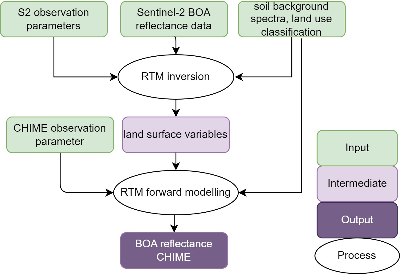
Figure 1: Overall workflow of simulating CHIME data based on Sentinel-2 data and Radiative Transfer Modelling (RTM).
Figure 1 illustrates the overall workflow used to simulate CHIME data based on Sentinel-2 observations and RTM. It is assumed that similar to Sentinel-2, CHIME will provide BOA reflectance products as analysis-ready data for end users. Consequently, BOA reflectance is selected as the target level for the representative dataset. Access to Level-1B and Level-1C products is only required for advanced applications involving user-defined atmospheric correction procedures (Rast et al., 2021).
To retrieve land surface parameters and perform the forward simulations, the Vista processing framework employs the integrated soil–leaf–canopy (SLC) reflectance model (Verhoef & Bach, 2007) to analyze the input reflectance spectra (e.g. Sentinel-2).
Besides from Sentinel-2 BOA reflectance SLC also needs the Sentinel-2 observation parameter (e.g. date & time of acquisition, atmospheric visibility, observation angles), soil background spectra from spectral libraries and derived scene specific soil spectra from Sentinel-2 data, as well as land use and cloud/cloud shadow classification. The soil background spectra used were obtained from the ECOSTRESS Spectral Library (Meerdink et al., 2019, Baldridge et al. 2009) as well as from own measurements.
While the SLC model is specialized on the retrieval of vegetation parameters, it is also capable of modelling soil, artificial surfaces, water bodies, and snow. Since the representative dataset is tailored towards the derivation of agricultural applications, vegetation parameters are deemed the most important. Nevertheless, with SLC it is possible to simulate complete CHIME scenes. Only clouds and cloud shadows, which are considered invalid pixels, are masked in the final dataset. To do so, SLC is used in a forward mode: the inverted vegetation and land surface parameters, CHIME observation parameters (e.g. date & time of acquisition, spectral resolution, observation angles) and soil background spectra as well as land use and could/cloud shadow masks are needed.
2.2. LSTM
The simulation of the representative Land Surface Temperature (LST) Monitoring (LSTM) mission LST is based on the Data Mining Sharpener (DMS) (Gao et al., 2012), which was implemented in the ESA-funded Sen-ET workflow (Guzinski et al., 2020). The DMS thermally sharpens Sentinel-3 (S3) Sea and Land Surface Temperature Radiometer (SLSTR) LST data using cloud-free Sentinel-2 (S2) MSI optical imagery and a Copernicus Digital Elevation Model (DEM). The DMS derives relationships between thermal and optical data at low resolution through a bagging algorithm of decision trees. In our approach, each 1000 m resolution Sentinel-3 (S3) acquisition was matched with a corresponding 10-day 20 m resolution Sentinel-2 (S2) composite. Then, the S2 reflectance bands and DEM data gets resampled to the S3 grid at 1000 m to train the predictive model. Next, based on the original S2 and DEM, S3 LST is predicted at the higher 20 m resolution. To ensure consistency in energy representation, a final bias adjustment was applied between the original low-resolution (LR) and the resulting high-resolution (HR) LST outputs. For further methodological details, we refer the reader to the Sen-ET algorithm manual (DHI GRAS, 2020).
To assess and improve the quality of the HR LST, a cross-calibration step based on quasi-simultaneous ECOSTRESS observations is added. In this step, all S3-ECOSTRESS observation pairs, with a maximum time difference of ten minutes in acquisition time, for 2023 and 2024 are gathered and compared to derive a gain and offset, as described by Snyders et al. (2025). Subsequently, the gain and offset are applied to all S3 HR LST, resulting in a cross-calibrated dataset S3* HR LST.
Since the sharpening process enhances the spatial resolution of LST from 1 km to 20 m, it is subsequently resampled to 30 m to be in line with the expected nadir spatial resolution of the LSTM mission. All pixels with a viewing zenith angle (VZA) exceeding 30° were excluded to align with LSTM acquisition geometry (Koetz et al., 2021). Figure 2 provides a schematic overview of the procedure to simulate the LSTM LST.
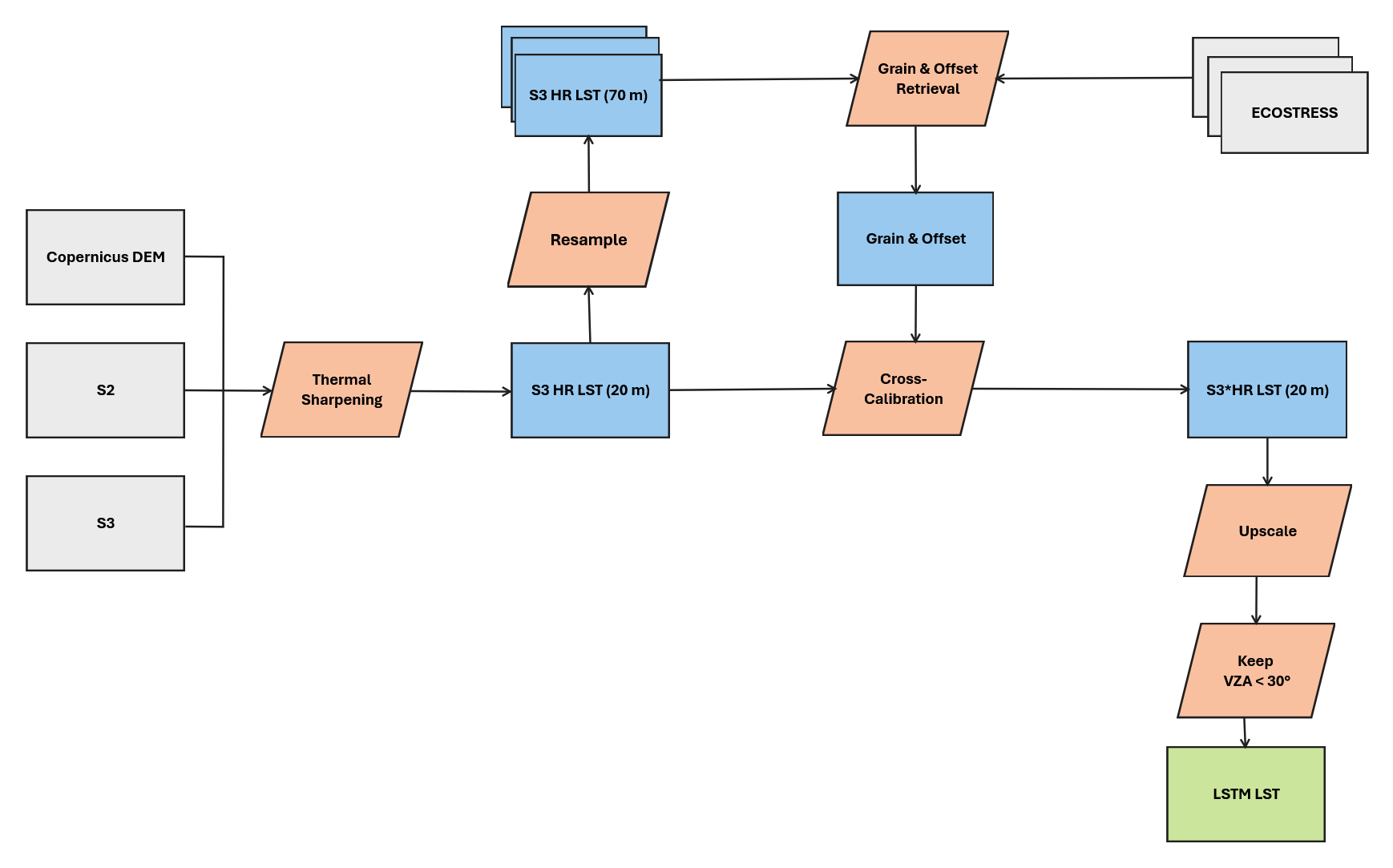
Figure 2: Processing flow for the representative LSTM dataset. Grey boxes, blue boxes and green boxes represent inputs, intermediates and outputs, respectively. Parallelograms represent process operations.
2.3. ROSE-L
The Radar Observing System for Europe in L-band (ROSE-L) representative dataset is synthesized from the SAtélite Argentino de Observación COn Microondas (SAOCOM)-1 L-band SAR data. By applying a consistent preprocessing workflow, SAOCOM-1 L1A stripmap data is transformed into products with spatial and radiometric characteristics that approximate those expected from ROSE-L.
SAOCOM-1 and the upcoming ROSE-L mission share key instrument characteristics that make such an approach feasible. The comparable frequency range of both missions makes SAOCOM-1 a suitable proxy for exploring change detection and coherence applications expected from ROSE-L. Although their antenna architecture and swath width differ, the core frequency range and polarimetric capabilities allow meaningful analogues to be drawn. Both operate in the L-band, ensuring comparable penetration depth. Both missions also offer full polarimetric capability, ensuring sensitivity to vegetation structure and soil conditions. The largest difference stems from the revisit period. The planned revisit period of the ROSE-L mission is 12 days (1 satellite) or 6 days (constellation). SAOCOM-1A and 1B satellites operate in a constellation regime, which allows using either an 8- or 16-day revisit cycle. However, due to the gaps in image acquisition and distribution plans, exact temporal coverage varies in different areas of interest.
In the next sections, we describe how SAOCOM-1 stripmap data can be processed to generate gamma nought (γ⁰) backscatter and coherence layers analogous to those expected from ROSE-L. Both datasets are computed by means of open-source ESA Sentinel Application Platform (SNAP) software (SNAP, 2025).
2.3.1. Backscatter
The backscatter computation workflow (Figure 3) begins with radiometric calibration, where the raw digital numbers are converted into terrain flattened γ⁰ backscatter. With terrain flattened γ⁰, we remove the radiometric variability associated with topography while leaving the radiometric variability associated with land cover (Small, 2011). Therefore, terrain flattened γ⁰ is particularly well suited for making results comparable between satellites of slightly different elevation heights.
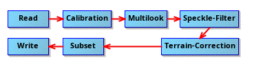
Figure 3: Processing workflow to derive γ⁰ backscatter from SAOCOM-1 L1A data product.
After calibration, multilooking is applied, averaging one pixel in range and two in azimuth direction to reduce speckle noise and geometric distortion. This step improves image interpretability at the cost of a slight reduction in spatial resolution. Speckle filtering follows, using the Refined Lee algorithm to further suppress noise while preserving structural details and edges.
Terrain correction is performed to geocode the data and correct for geometric distortions caused by SAR imaging geometry and topography. The Shuttle Radar Topography Mission (SRTM) 1 sec elevation model is used to terrain correct the imagery to 5 m pixel spacing in the target projection. Finally, a spatial subset is extracted based on a predefined geometry, reducing the dataset to the area of interest for further analysis.
2.3.2. Coherence
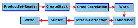
Figure 4: Processing workflow to derive 16-day coherence from SAOCOM-1 L1A products.
The processing workflow of coherence coefficient derivation (Figure 4) begins with the creation of a product pair, between which the coherence coefficient is computed. We consider two products as an eligible pair if they
- Share the orbit path number, i.e. they are from the same relative orbit;
- Have a temporal separation of 8 or 16 days;
- Spatially overlap of at least 33.3%.
The last requirement needs to be applied for proper co-registration. If the overlap is too small, the co-registration algorithm cannot align them. Due to the overlap of SAOCOM data products, it might happen that multiple pairs are formed for a given area. By applying the spatial overlap filter, the creation of pair duplicates is avoided. The exact value of the spatial overlap threshold was chosen by means of trial and error.
From the paired products, an interferometric stack is created, where the reference and secondary acquisitions are co-registered based on orbit information. Cross-correlation is then applied to refine the co-registration using ground control points and windowed matching, ensuring pixel-level alignment between the two images. The warp step resamples the secondary image to the geometry of the reference scene, correcting residual misregistration.
Once co-registration is complete, coherence estimation will follow. The interferometric coherence is computed over a moving window (10 × 10 pixels in both range and azimuth direction) after flat-Earth and topographic phase removal using the SRTM 1 sec elevation model. This step quantifies the similarity between the two SAR acquisitions, providing a direct measure of temporal decorrelation.
The resulting coherence map is then subjected to terrain correction, which geocodes the data and corrects geometric distortions using the SRTM 1 sec DEM and resamples the data to 5 m pixel spacing in the target map projection. Finally, a subset is extracted based on a predefined geometry, retaining only the area of interest for further analysis.
3. Results & Discussion
Representative datasets were generated over three agricultural regions in Belgium, Germany, and Estonia (Figure 5). The selected areas of interest (AOIs) correspond to Sentinel-2 tiles 31UFS (Belgium), 32UPC (Germany), and 35VMF (Estonia). These AOIs were chosen to represent a range of agro-climatic and land-use conditions.
The simulated datasets are publicly available in the ESA Project Results Repository (Application Propagation Environments / APEx: https://apex.esa.int/) as collections per Copernicus Sentinel Expansion Mission (VISTA, 2026; VITO, 2026; KappaZeta, 2026).
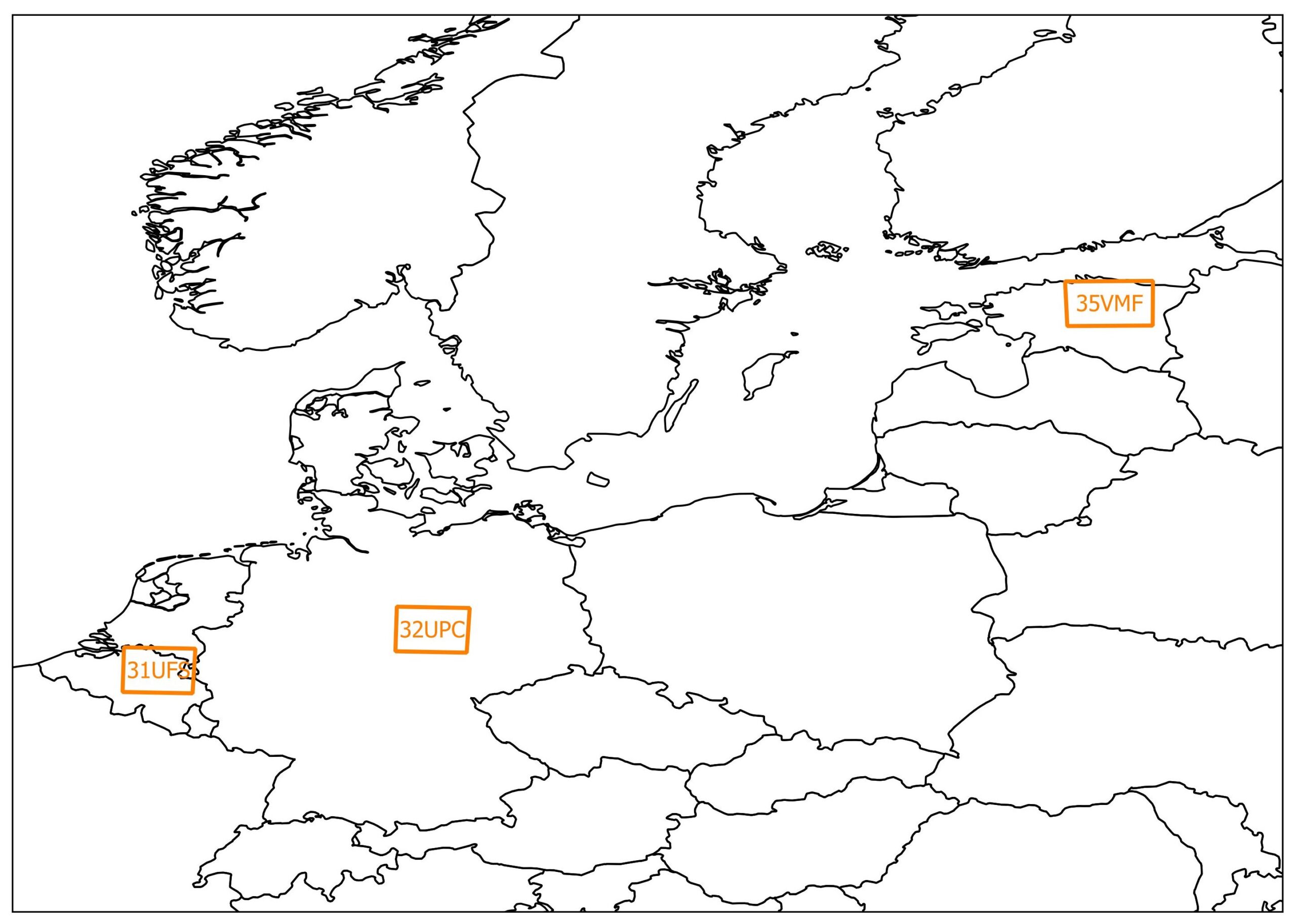
Figure 5: AOIs based on the extent of Sentinel-2 tiles in Belgium (31UFS), Germany (32UPC), and Estonia (35VMF), country boarders from Sandvik (2008).
3.1. CHIME
The simulated CHIME datasets for the three AOIs and the years 2024 and 2025 reflect the currently expected sensor characteristics. The spectral coverage spans 450–2450 nm, sampled in 197 contiguous spectral bands, while the spatial resolution is 30 m × 30 m. Each simulated scene covers an area of approximately 110 km × 110 km, closely matching the anticipated CHIME swath geometry. Sensor noise was not explicitly added during the simulation, as the Sentinel-2 input data already contain realistic noise characteristics, and the final CHIME signal-to-noise ratio specifications are not yet fully defined.
The period for which scenes were generated was set from March 1st to November 30th in both years. In total, 20 CHIME scenes were generated for the AOI in Germany in 2024 and 23 scenes in 2025. For the Estonian AOI, 20 and 21 scenes were generated, respectively, while for the Belgian AOI, 18 and 22 scenes were produced. All scenes are provided as cloud-optimized GeoTIFFs (COGs) along with the corresponding metadata in XML format. Figures 6 and 7 exemplarily show the availability of CHIME scenes for the German AOI in the years 2024 and 2025.

Figure 6: Availability of CHIME scenes in the German AOI for the year 2024.

Figure 7: Availability of CHIME scenes in the German AOI for the year 2025.
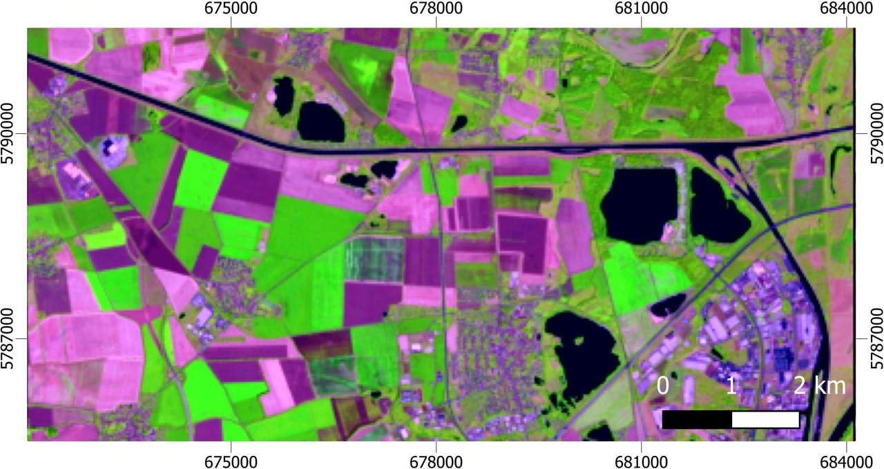
Figure 8 shows representative reflectance spectra extracted from the simulated CHIME dataset for different surface types within AOI 32UPC on 30 July 2024, demonstrating physically plausible spectral behavior across the visible, near-infrared, and shortwave infrared domains. A qualitative spatial comparison is shown in Figures 9 and 10, where a Sentinel-2 false-color composite acquired on 29 July 2024 is compared with the corresponding simulated CHIME scene. Despite differences in spectral sampling and spatial resolution, the simulated CHIME data preserve major spatial patterns and land-cover structures.
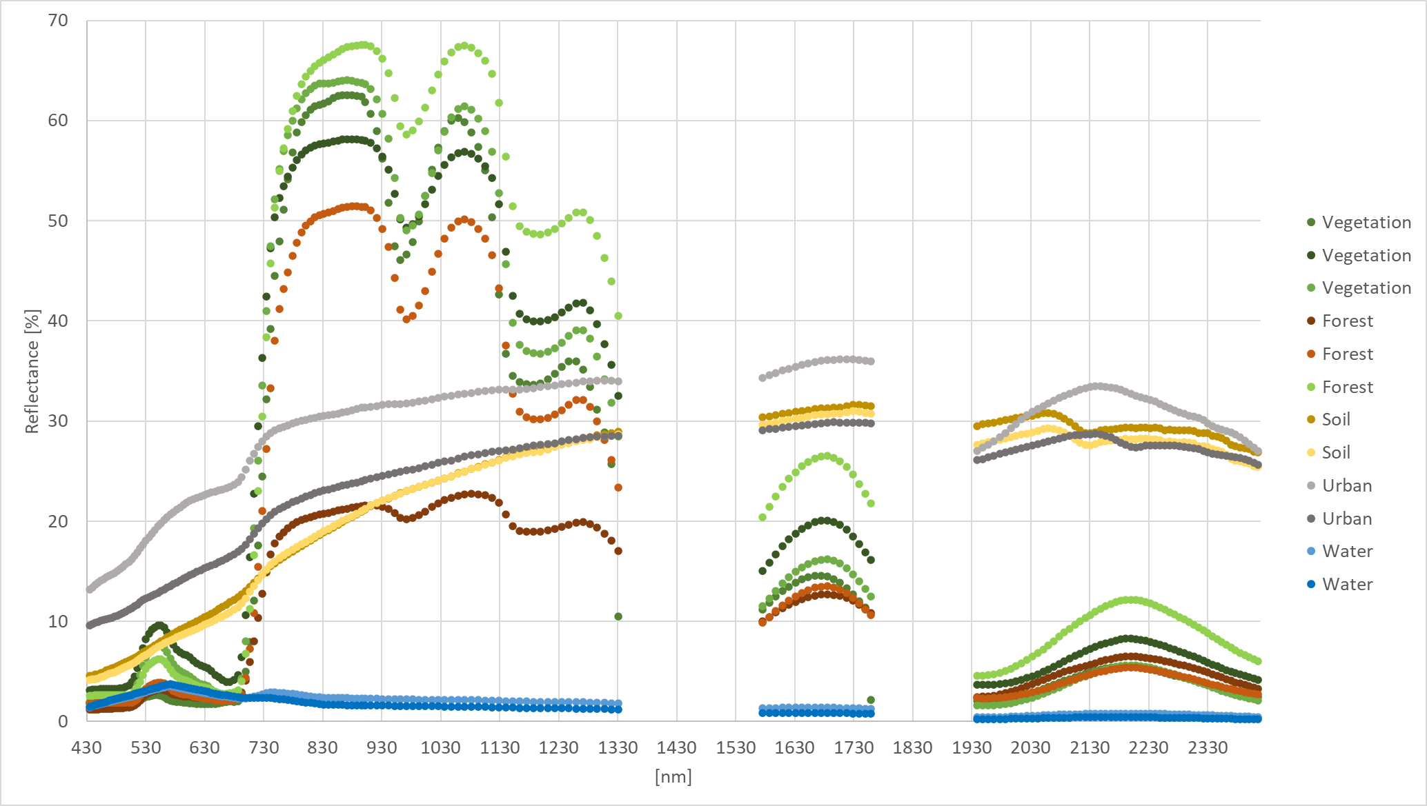
Figure 8: Sample spectra from simulated CHIME data of different surface types from AOI 32UPC, 13.05.2024.
Figure 9 shows a section of the 32UPC Sentinel-2 scene from 29.07.2024 in false colors, and Figure 10 shows the corresponding section in the simulated CHIME data set.
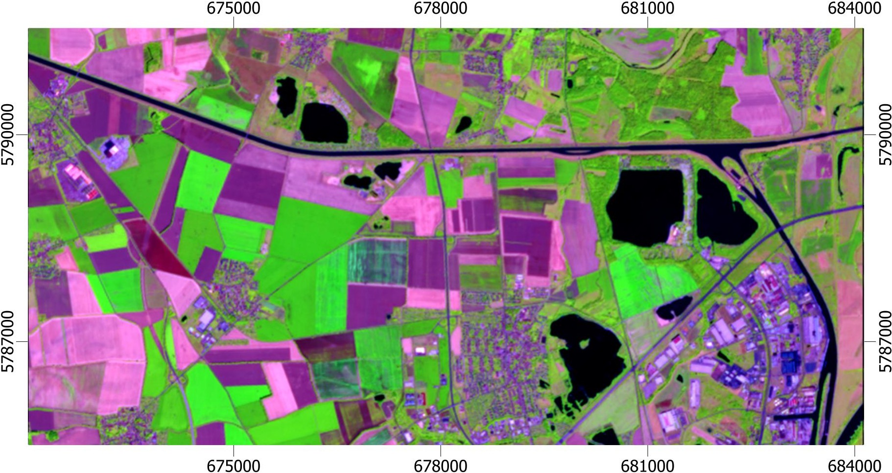
Figure 9: Original Sentinel-2 32UPC image on Jul 29th 2024 in false color combination (664nm, 864nm, 1614nm). Coordinate System: WGS 84 UTM zone 32N
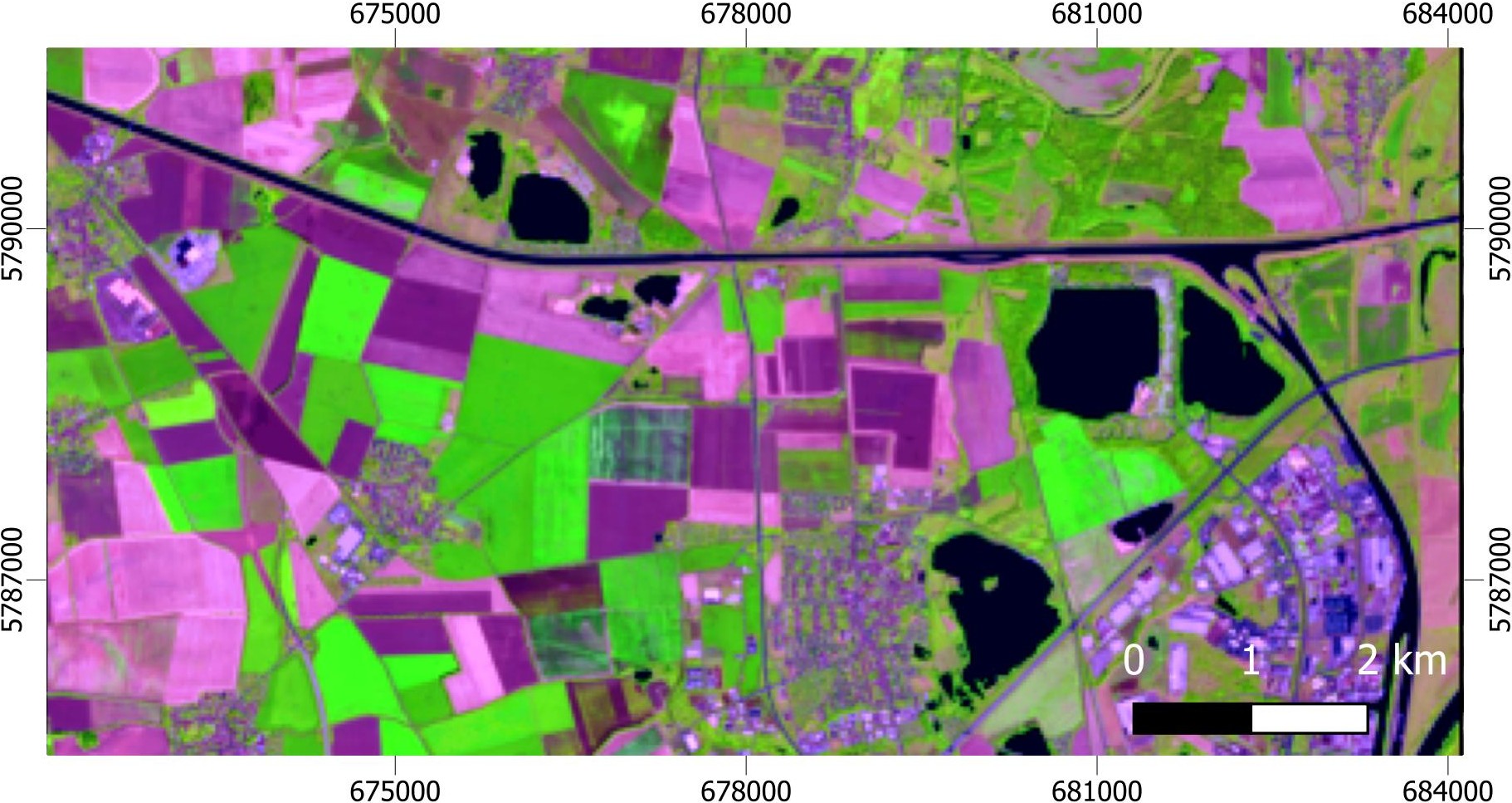
Figure 10: Simulated CHIME image in false colour combination (667nm, 864nm, 1609nm) and 30m spatial resolution. Coordinate System: WGS 84 UTM zone 32N
Quantitative validation of the simulated CHIME reflectance values was performed using hyperspectral observations from EnMAP. BOA reflectance values from the simulated CHIME dataset were compared against EnMAP reflectance acquired over the same AOI within a maximum one-day temporal offset. Table 2 summarizes all simulated CHIME scenes and corresponding EnMAP acquisitions available for AOI 32UPC in 2024.
In total, 16 simulated CHIME scenes and 8 EnMAP acquisitions were initially available. After filtering for cloud contamination and temporal proximity, only two acquisition periods were suitable for validation: 13–14 May 2024 (three EnMAP tiles) and 29–30 July 2024 (two EnMAP tiles). The scene-pair selection procedure and exclusion criteria are detailed in Table 2, with cloud cover being the primary limiting factor. The scene-pairs highlighted in green were selected for validation.
Table 2: Data availability and scene-pair selection for validation of AOI 32UPC.
| CHIME scene dates | Suitable EnMAP acquisiton dates | Selected for Validation? | Comments |
| 19.03.2024 | 17.03.2024 | No | Cloud cover in CHIME and EnMAP data |
| 31.03.2024 | – | No | No EnMAP data near to CHIME date |
| 08.04.2024 | 17.04.2024 | No | Cloud cover in EnMAP data |
| 30.04.2024 | No | ||
| 13.05.2024 | 10.05.2024 | No | No area overlap |
| 14.05.2024 | Yes | 3 scenes from EnMAP data are selected | |
| 23.05.2024 | No | Dates are too far apart | |
| 12.06.2024 | – | No | No EnMAP data near to date |
| 27.06.2024 | 07.07.2024 | No | Cloud cover in EnMAP data |
| 07.07.2024 | No | ||
| 19.07.2024 | 30.07.2024 | No | Days are too far apart |
| 29.07.2024 | Yes | 2 out of 3 scenes from EnMAP data are cloud-free and selected | |
| 03.08.2024 | No | Cirrus and cloud cover in EnMAP data | |
| 11.08.2024 | No | ||
| 21.08.2024 | 30.08.2024 | No | Cloud cover in CHIME data Cloud cover in CHIME data |
| 02.09.2024 | No | ||
| 12.09.2024 | – | No | No EnMAP data near to CHIME dates |
| 22.09.2024 |
For validation, several metrics were used. The selected metrics are standard and widely used in hyperspectral image validation and inter-sensor comparison studies:
- Mean Spectral Difference (MSD) [%]: Mean absolute difference between CHIME and EnMAP pixels’ reflectance for each spectral band, as well globally across all bands.
- Root Mean Squared Error (RMSE) [%]: Square root of the mean squared pixel-wise difference between CHIME and EnMAP reflectance for each band, as well as globally across all bands.
- Structural Similarity Index (SSIM): Quantifies similarity between CHIME and EnMAP data in terms of structure, luminance, and contrast for each spectral band (Wang et al., 2004). SSIM is unitless and in the range of [0,1], with 1 indicating perfect similarity.
- Correlation Coefficient: Measures the linear / Pearson correlation between CHIME and EnMAP pixel reflectance values for each band, as well as globally across all bands. Correlation is unitless and in the range of [-1,1], with values closer to 1 indicating stronger linear relationship. The spectral correlation maps in Figures 11, 12, 13a retain the full [−1, 1] range to capture spatial anomalies at the pixel level, whereas the dual-axis plot in Figure 14 is restricted to [0, 1] because only positive, physically meaningful correlations are observed in the aggregated band-wise metrics.
- Spectral Angle Mapper (SAM) (radians): Computes the spectral angle between CHIME and EnMAP spectra to assess spectral shape similarity (Kruse et al., 1993). Smaller SAM indicates a better match.
- Spectral Information Divergence (SID): Measures spectral dissimilarity by comparing probability distributions derived from CHIME and EnMAP spectra (Chang et al., 2000). SID is unitless and is treated as a score, with lower values meaning greater similarity.
As clouds and cloud shadows are not considered, available masks from the EnMAP and Sentinel-2 data were combined (Cloud mask, cloud shadow mask, haze mask, cirrus mask). However, it is to be noted that some cloud and cloud shadow regions are not completely detected and flagged in these available masks.
Overall, five scene-pairs are validated, and the aggregated results of the global metrics are reported in Table 3. MSD and RMSE indicate moderate radiometric differences, while low SAM and SID values, together with high correlation coefficients (≥ 0.89, average 0.924), demonstrate strong spectral consistency between CHIME and EnMAP. SID values remain almost always below 0.05, which is commonly regarded as indicative of good spectral agreement in hyperspectral analysis as per discussions in van der Meer (2006) while SAM values in the range of 0.1–0.15 radians suggest only moderate spectral deviation.
Table 3: Global spectral validation metrics between CHIME and EnMAP for five matched scenes pairs in AOI 32UPC.
| Dates | Scene Pair | MSD [%] | RMSE [%] | SAM (radians) | SID | Correlation |
| CHIME: 13.05.2024 EnMAP: 14.05.2024 | 1 | 3.90 | 6.21 | 0.133 | 0.055 | 0.939 |
| 2 | 4.42 | 6.46 | 0.135 | 0.044 | 0.932 | |
| 3 | 3.91 | 5.97 | 0.105 | 0.038 | 0.955 | |
| CHIME: 29.07.2024 EnMAP: 30.07.2024 | 4 | 3.67 | 5.49 | 0.144 | 0.038 | 0.909 |
| 5 | 4.48 | 6.64 | 0.162 | 0.054 | 0.887 | |
| Average | 4.076 | 6.154 | 0.136 | 0.046 | 0.924 |
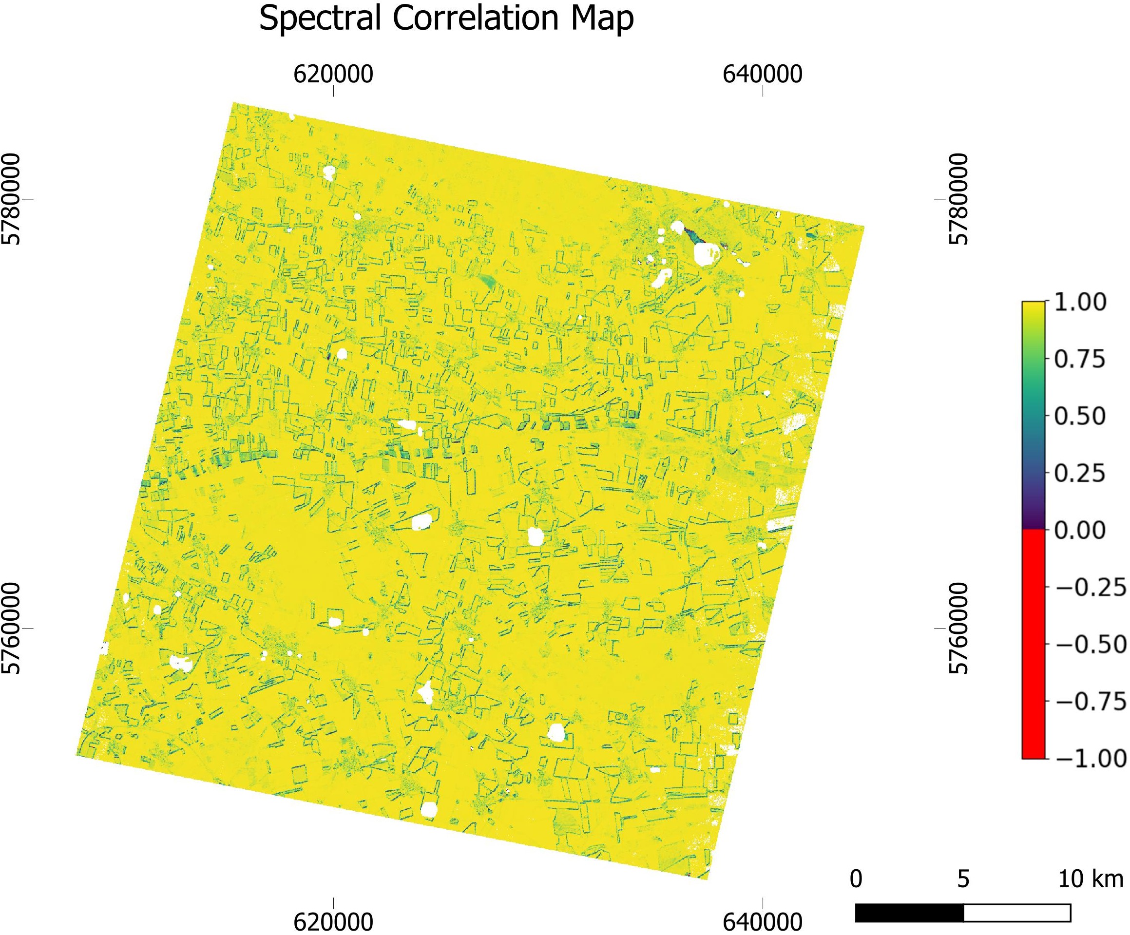
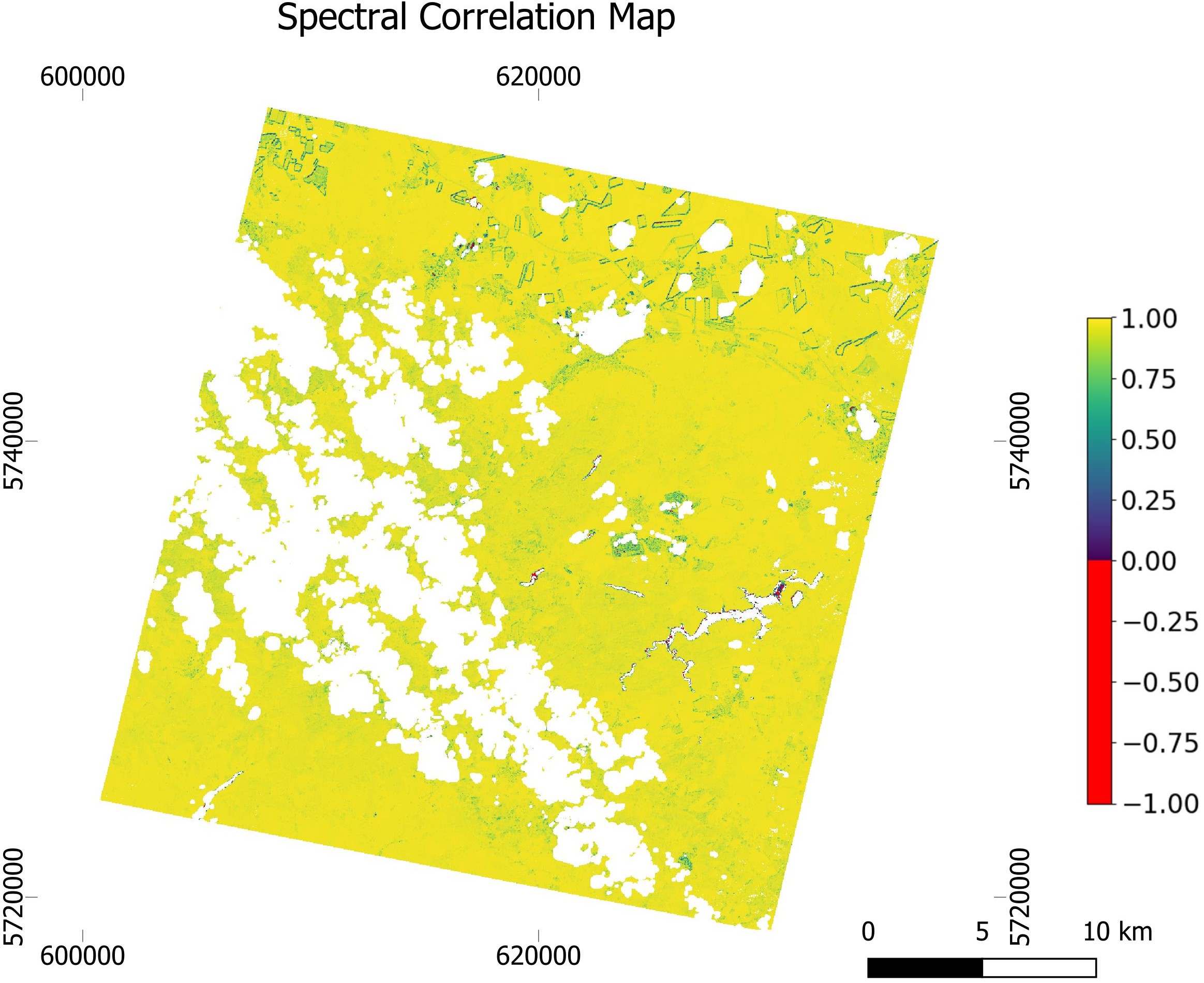
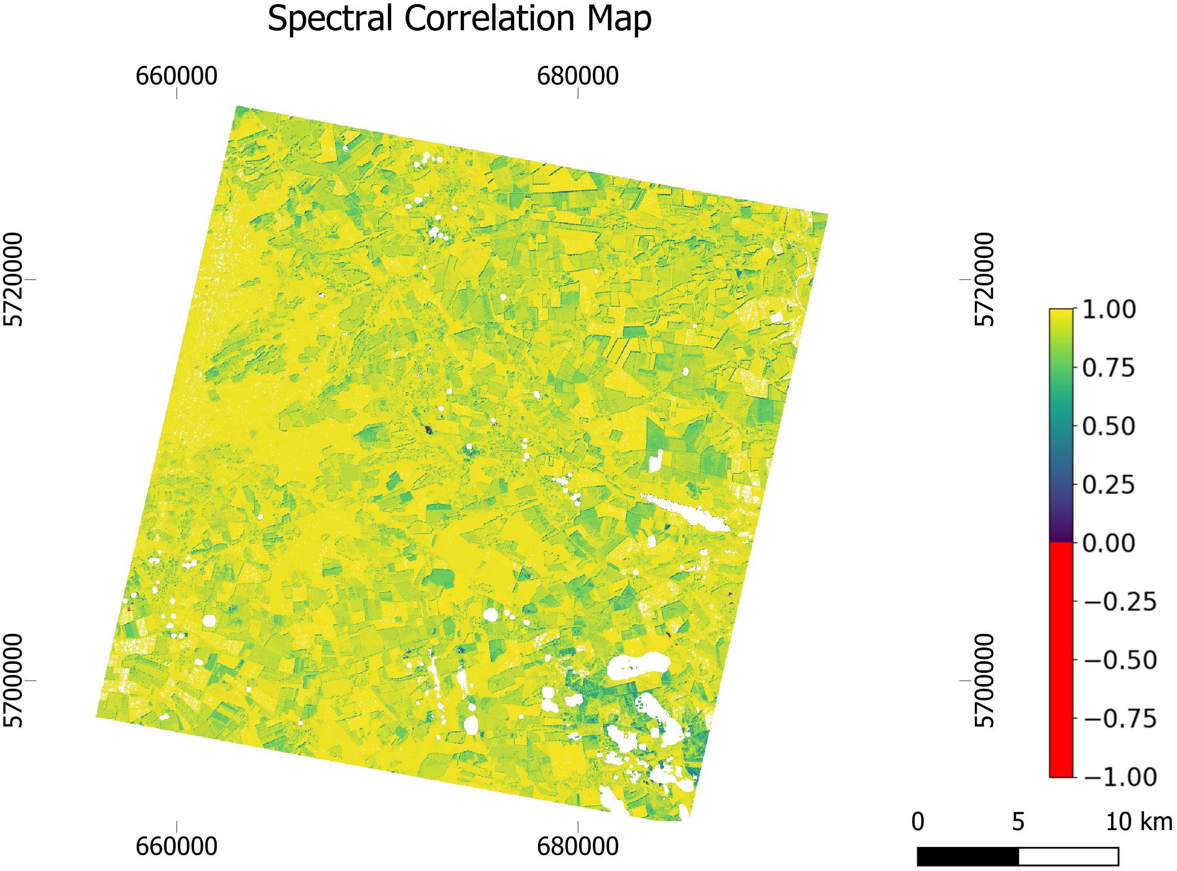
Pixel-wise spectral correlation maps (see Figures 11, 12, 13a) show predominantly high agreement between CHIME and EnMAP across the scenes. Yellow regions correspond to near-perfect correlation (close to 1), indicating strong spectral consistency, particularly over land and vegetated areas that are the primary focus of the representative CHIME dataset. The spatial distribution of spectral correlation does not show an evident association with specific land-use or crop types. In contrast, green to blue regions represent reduced correlation values (approximately 0.5 or lower) and are spatially localized rather than systematic. White regions are excluded for validation via cloud-related masks. Red regions show areas with negative correlation, implying the existence of some inverted pixel spectra.
Figure 11 illustrates areas of reduced correlation along object boundaries and fine spatial structures, which can be attributed to resolution mismatch and slight geolocation misalignment between the two sensors. These effects are most pronounced at sharp edges (e.g., urban features or field boundaries), where small spatial offsets lead to pixel-wise spectral differences despite overall scene-level consistency. Figure 12 highlights water bodies, where lower correlation values are observed. These regions are not a primary focus of the representative CHIME dataset nor of the dataset generation methodology, which is designed to capture and validate spectral consistency over land surfaces and vegetation areas. Consequently, the observed behavior over water does not reflect deficiencies in the generated dataset.
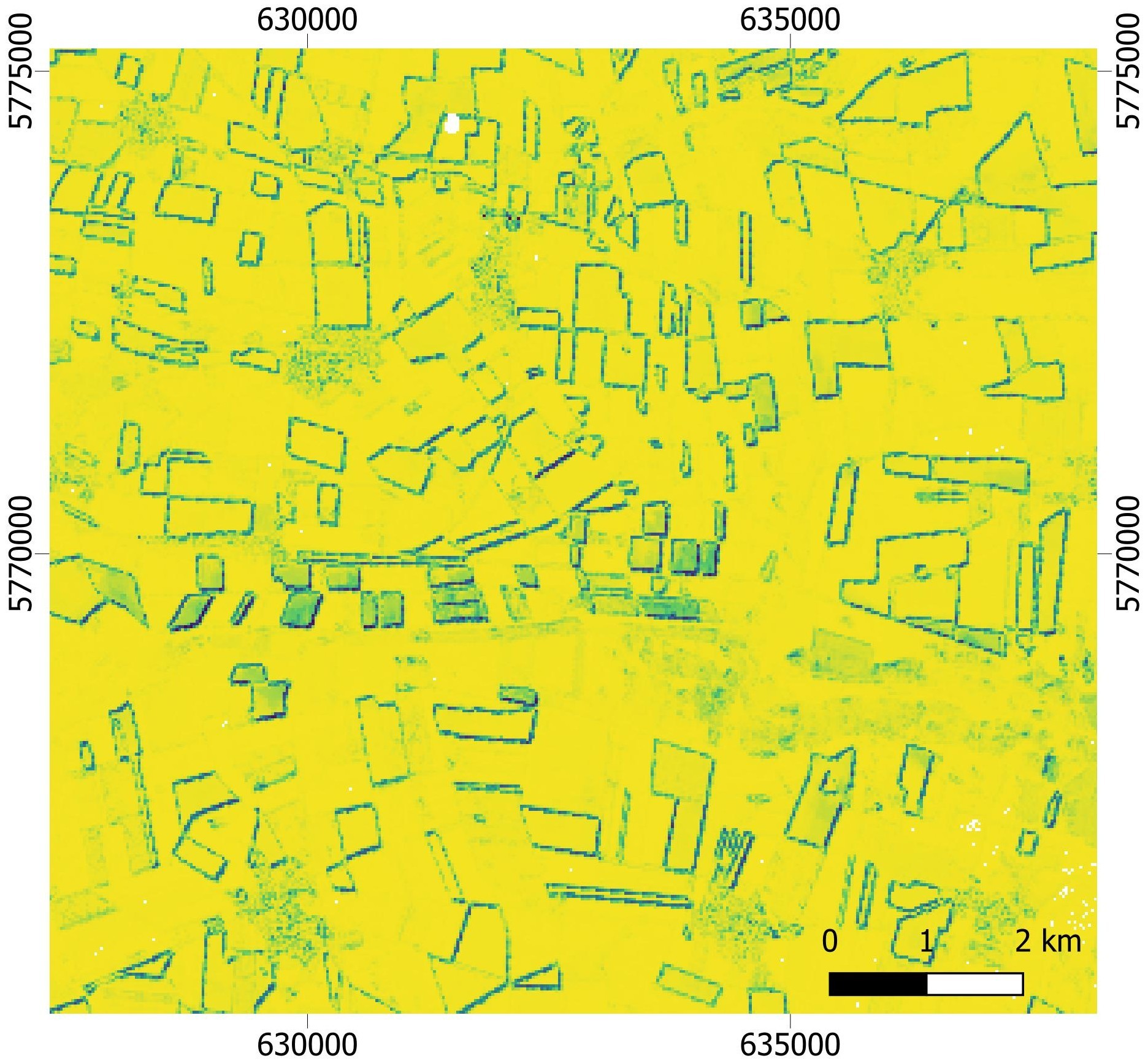
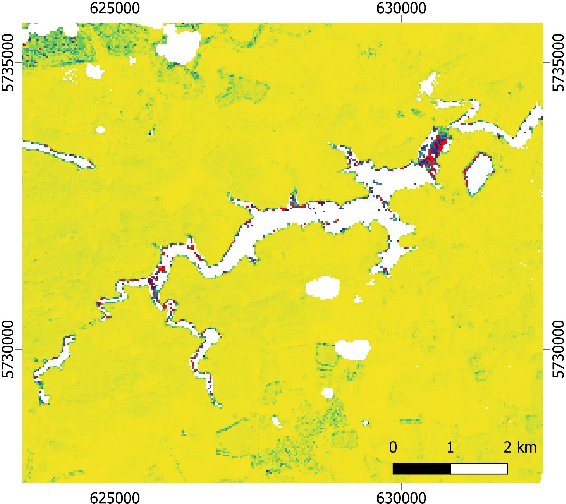
Figure 11: Spectral Correlation between CHIME Figure 12: Spectral Correlation between CHIME (13.05.2024) and EnMAP (14.05.2024) of an area (13.05.2024) and EnMAP (14.05.2024) of an area in in 32UPC (Scene Pair 1). Coordinate System: 32UPC (Scene Pair 2). Coordinate System: WGS 84 UTM zone 32N WGS 84 UTM zone 32N
Figure 13a shows regions affected by cirrus clouds and cloud shadows. The accompanying EnMAP reference Figure 13b demonstrates that these atmospheric features were not fully detected by the applied cloud masks, resulting in localized reductions in correlation. These effects are attributable to residual atmospheric contamination rather than limitations of the CHIME dataset generation approach.
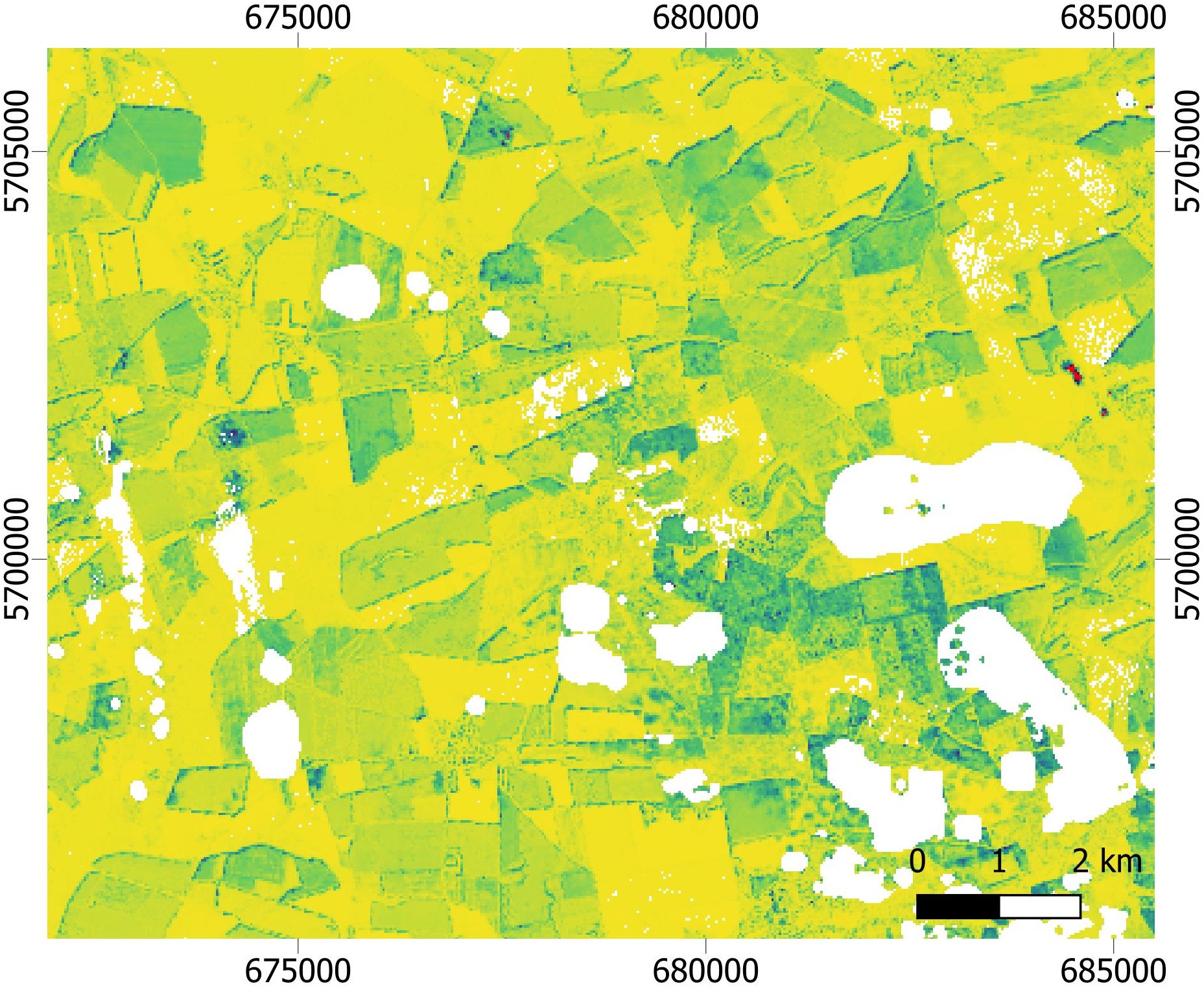
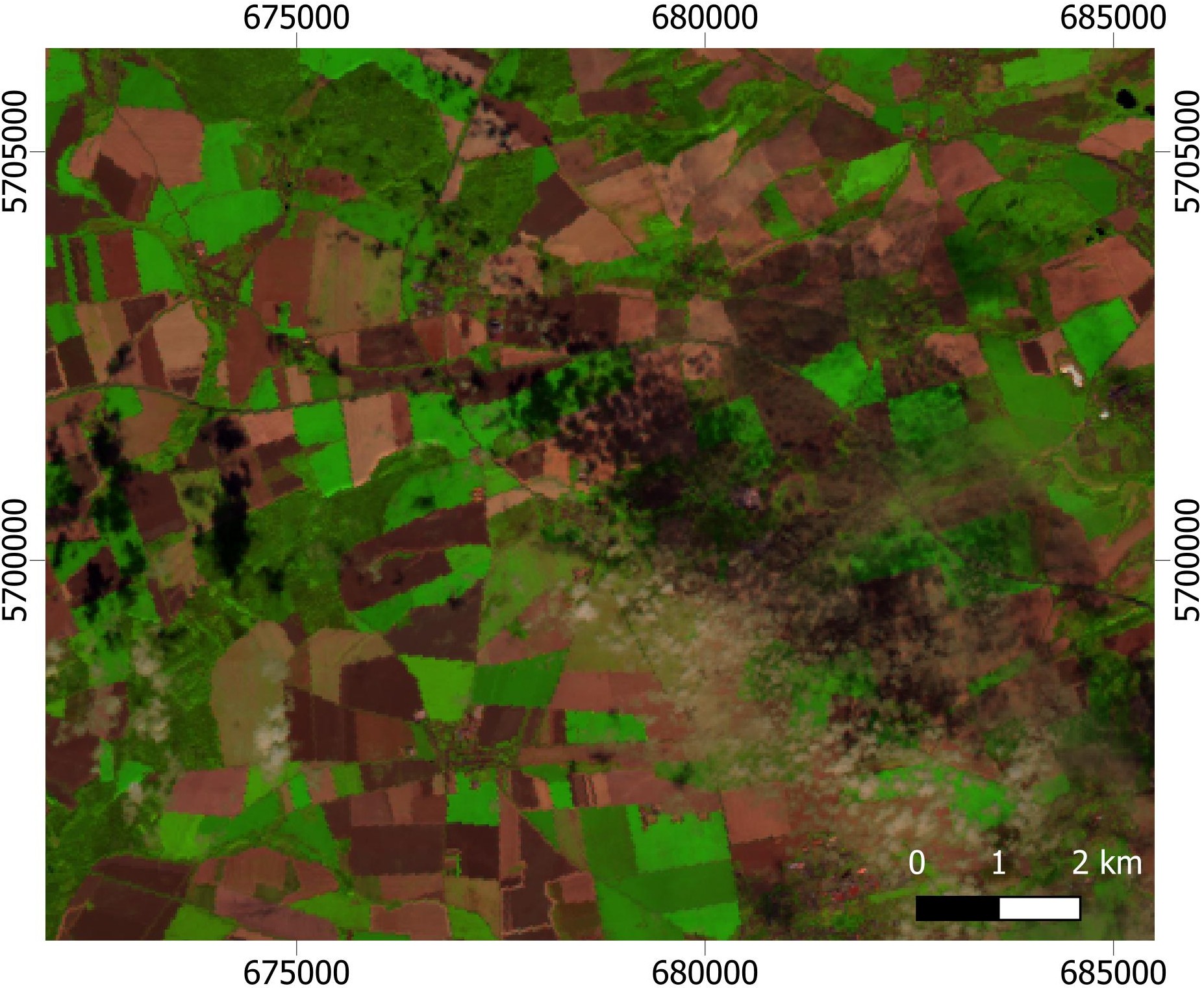
Figure 13: (a) Spectral Correlation between CHIME (29.07.2024) and EnMAP (30.07.2024) of an area in 32UPC (Scene Pair 5) (b) Corresponding cirrus cloud and cloud shadow coverage in EnMAP data. Coordinate System: WGS 84 UTM zone 32N
Overall, the spatial correlation patterns confirm that the generated dataset exhibits high spectral fidelity over land and vegetation surfaces, while localized reductions in correlation are well explained by known effects related to resolution differences, surface type, and incomplete cloud masking, and do not diminish the overall quality or intended use of the dataset. For spectral correlation maps of all validated scene pairs, see Appendix A.
Figure 14 displays an overall density-based comparison between CHIME (13.05.2024) and EnMAP (14.05.2024) reflectance values for Scene Pair 3, obtained from random sampling across all spectral bands. Each point represents a valid pixel-band pair, while the kernel density estimates highlight regions of high sample concentration. The black 1:1 line indicates perfect radiometric agreement, whereas the red regression line represents the cross-calibration relationship between both datasets. The strong alignment along the 1:1 line confirms overall radiometric consistency despite temporal and atmospheric differences between acquisitions. The highest density of samples occurs at low reflectance values, reflecting the dominance of darker surface types such as water bodies, shadows, and low-reflectance vegetation within the scene. The increasing spread of the density distribution toward higher reflectance values indicates larger variability for brighter targets, which is expected due to differences in atmospheric correction, bidirectional reflectance effects, and temporal mismatch between acquisitions.
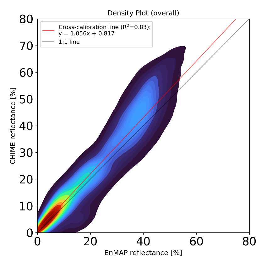
Figure 14: Density plot of CHIME (13.05.2024) and EnMAP (14.05.2024) for Scene Pair 3 in AOI 32UPC
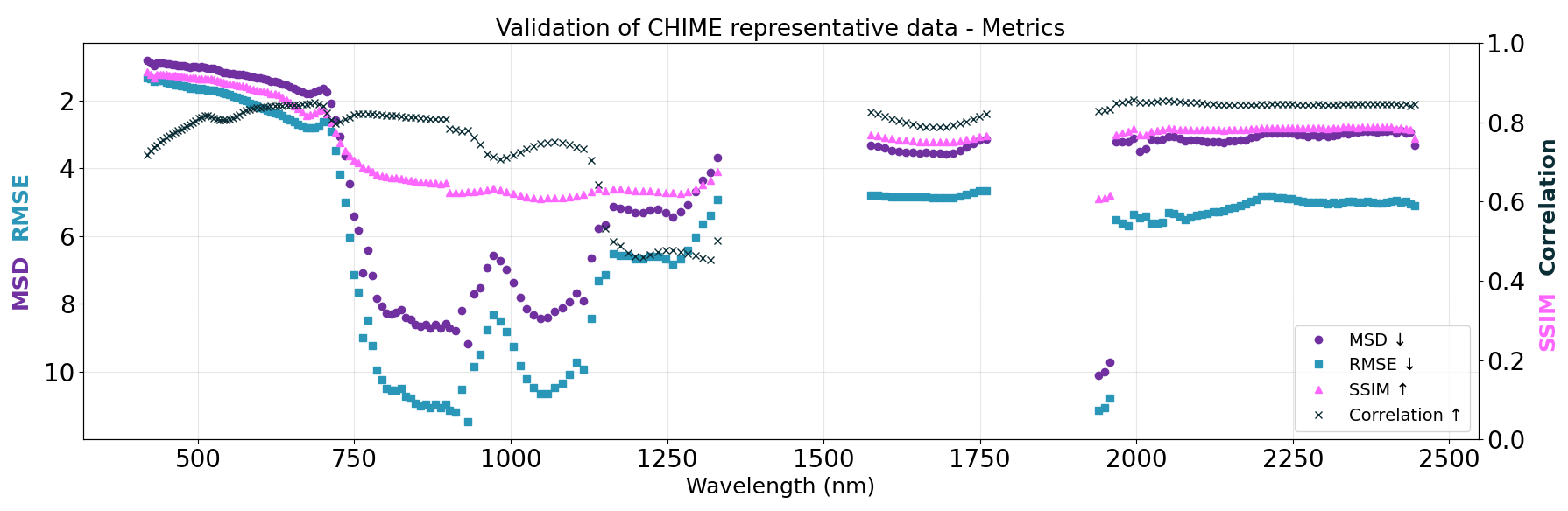
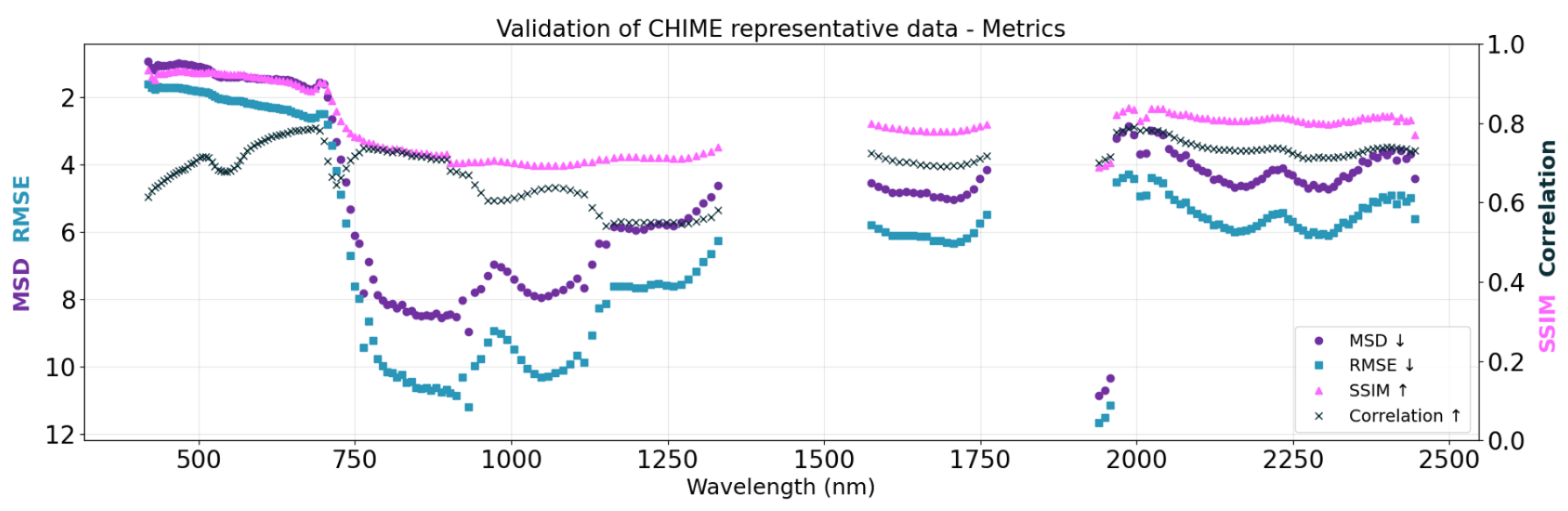
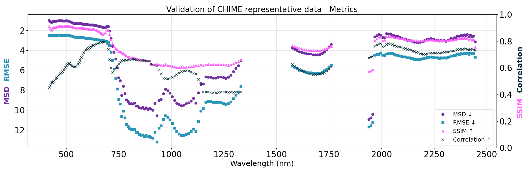
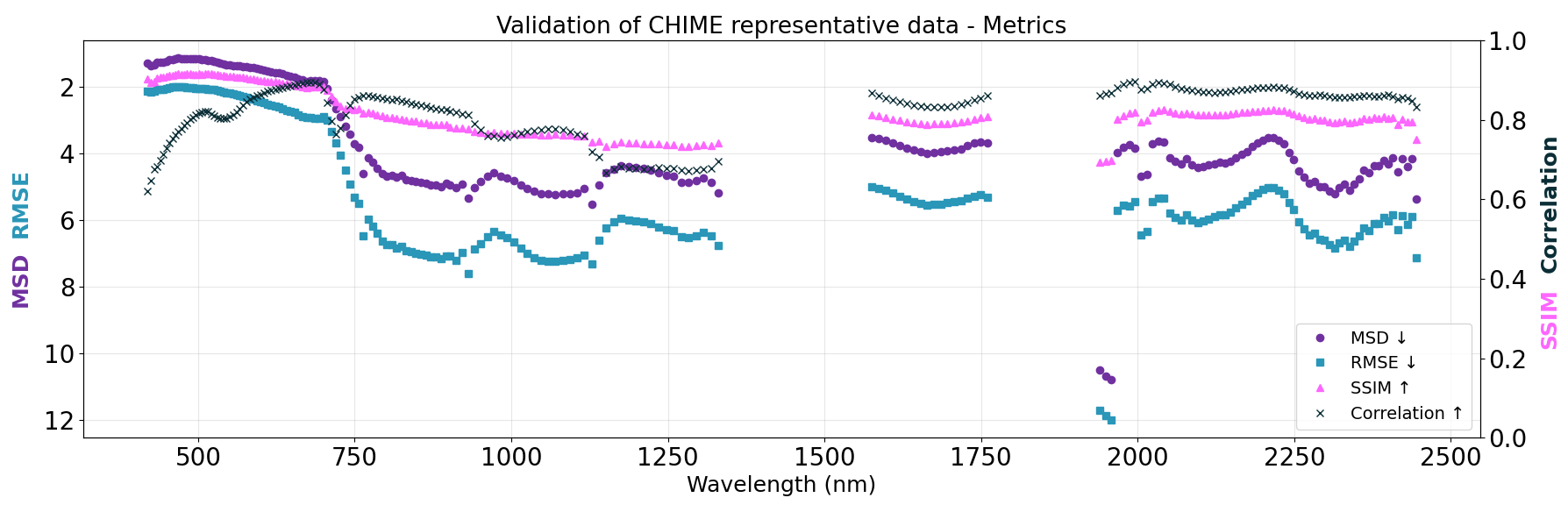
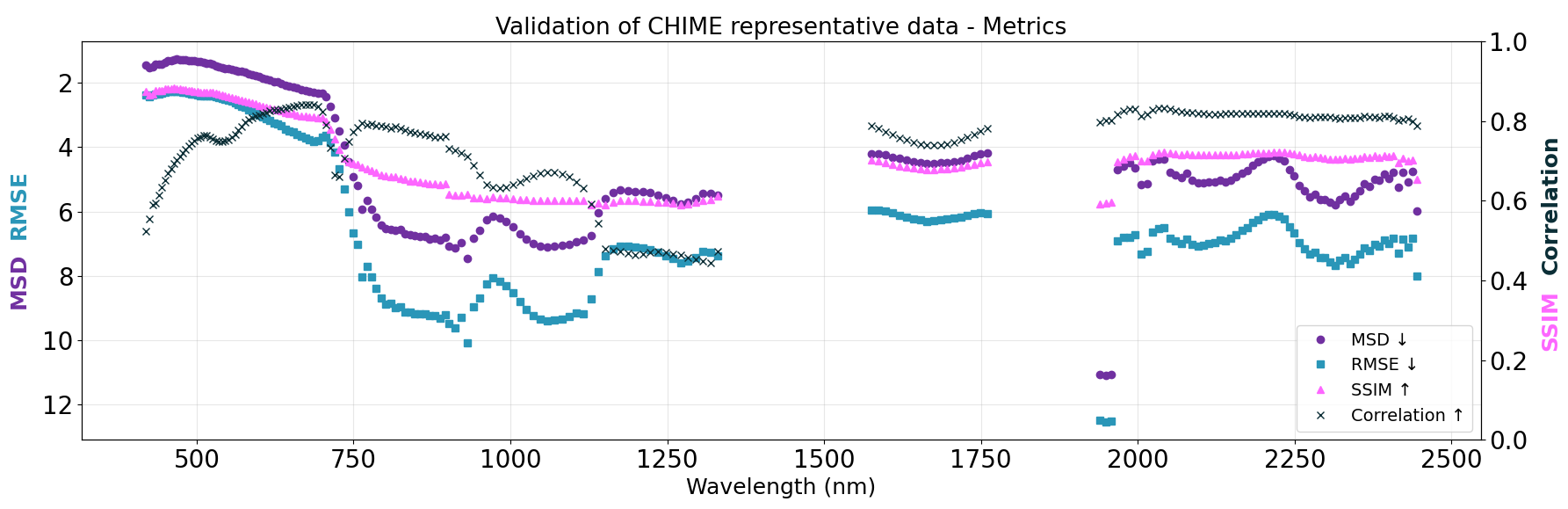
Figure 15 shows the per-band validation metrics between CHIME (13.05.2024) and EnMAP (14.05.2024) for the same Scene Pair 3. MSD and RMSE (left inverted axis) highlight absolute radiometric discrepancies, while consistently high SSIM and Correlation (right axis) across most wavelengths indicate strong structural agreement. The global correlation was computed by concatenating all valid pixel–band observations into two vectors and evaluating the Pearson correlation coefficient across this pooled dataset. In contrast, the band-wise correlations were computed independently for each spectral band, using only the spatial variation within that wavelength. As a result, the global correlation reflects both within-band spatial covariance and between-band spectral covariance, effectively capturing the joint structure of the data across spatial and spectral dimensions. The high global values indicate strong overall agreement in the combined distribution of reflectance values, including consistency in the relative magnitude and ordering of spectral responses across bands. The band-wise correlations, on the other hand, isolate the spatial correspondence at fixed wavelengths and therefore provide a more localized view of agreement that can vary across the spectrum. The observed difference between the global and band-wise correlations is expected, as the two metrics quantify correlation over different statistical domains and are not directly comparable as simple averages.
The observed pattern in the near-infrared plateau is primarily attributed to differences in atmospheric water vapor and/or plant water content. As the validation data are not acquired at the same time as the simulated CHIME data, variations in vegetation water status and atmospheric conditions are expected and represent a realistic source of discrepancy, thereby influencing the validation metrics. Isolated peaks in RMSE and MSD, together with reduced SSIM and correlation values around 1950 nm, are most likely associated with residual atmospheric effects in the EnMAP images in this strong water absorption region. Validation of other scenes also shows a similar pattern of increased MSD and RMSE at the same wavelength ranges (see Appendix A).
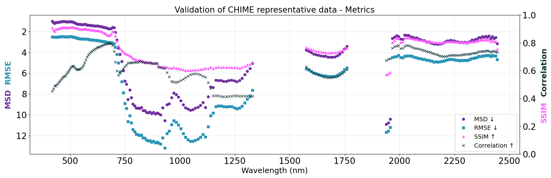
Figure 15: Per-band validation metrics of CHIME (13.05.2024) and EnMAP (14.05.2024) across the wavelengths for Scene Pair 3 in AOI 32UPC.
The validation results indicate that the proposed simulation framework can generate CHIME-like hyperspectral BOA reflectance data that are spectrally and spatially consistent with EnMAP observations. High correlation coefficients, low SID values, and moderate SAM values across all validated scenes demonstrate that the simulated data preserve spectral shape and relative radiometric behavior despite being derived from multispectral Sentinel-2 inputs.
The observed radiometric differences, reflected by MSD and RMSE, are within the expected range for inter-sensor comparisons and can largely be attributed to differences in spatial resolution, and acquisition geometry, as well as to increased uncertainty in atmospheric absorption regions and the SWIR domain. Localized discrepancies are mainly associated with residual cloud contamination and non-vegetated surfaces, which are of limited relevance for the vegetation-focused representative dataset.
The omission of an explicit CHIME-specific noise model results in a best-case representation of data quality and is considered appropriate for pre-launch algorithm development and sensitivity analyses.
Overall, the results demonstrate that the simulated CHIME dataset is sufficiently realistic to support pre-launch algorithm development and validation. The strong spectral agreement with EnMAP suggests that downstream retrievals of vegetation-related biophysical parameters can be expected to perform reliably under anticipated CHIME observation conditions.
3.2. LSTM
3.2.1. Cross-Calibration
The cross-calibration is based on quasi-simultaneous S3-ECOSTRESS LST pairs during 2024 and 2025 for tiles 31UFS and 32UPC. Tile 35VMF is not considered due to the lack of ECOSTRESS data for latitudes above 52°. Figure 16 shows the pixel-by-pixel comparison of all acquisition pairs for the relevant period and tiles. As the figure shows a strong resemblance between the two datasets, the cross-calibration is not relevant and thus obsolete. Instead, the ECOSTRESS data serves directly as validation data.
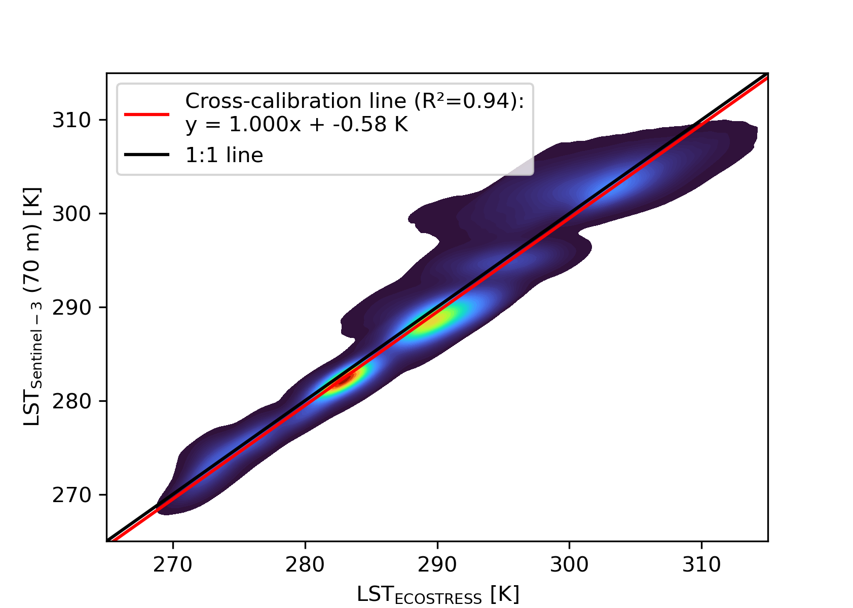
Figure 16: Density plot of LST comparison between high-resolution S3 LST and ECOSTRESS LST at 70m for all quasi-simultaneous observation pairs in 2024 and 2025 for tiles 31UFS and 32UPC.
3.2.2. LSTM dataset
For the representative LSTM dataset, all S3 and S2 acquisitions from 2024 and 2025 were downloaded for the AOIs: 31UFS, 32UPC, and 35VMF. Since the DMS generates LSTM-like LST files for each S3 acquisition, the resulting dataset includes files for all S3 acquisition times—provided both the S3 acquisition and the S2 composite contain cloud-free pixels. Consequently, LSTM-like files are generated daily, typically in the morning around 10:00 and in the evening around 22:00. In some cases, SLSTR captures the AOI with two acquisitions within a few minutes of each other. This might result in four LSTM files in one day in some cases. Since the planned acquisition time of the future LSTM mission will be around midday in Europe, the morning acquisitions (i.e. around13:00 UTC) are considered the most representative of the future mission characteristics.
The final LSTM dataset for the year 2024 comprises 698, 799, and 805 files for 31UFS, 32UPC, and 35VMF tiles, respectively. For the year 2025 the final LSTM dataset comprises 821, 830, and 802 files for 31UFS, 32UPC, and 35VMF tiles, respectively. It is important to note that each crop field within the AOIs is observed significantly fewer times due to cloud cover and incomplete spatial coverage during acquisitions. Figures 17 and 18 exemplarily show the availability of LST products for the German AOI 32UPC in the years 2024 and 2025.

Figure 17: Availability of LST product scenes in the German AOI for the year 2024.

Figure 18: Availability of LST product scenes in the German AOI for the year 2025.
Figure 19 illustrates an example of an LSTM-like LST acquisition for tile 32UPC.
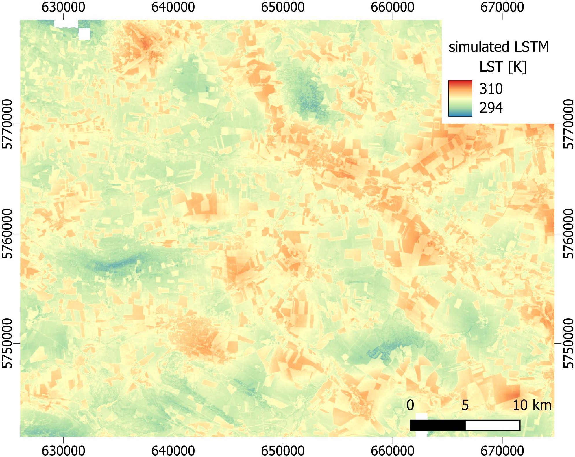
Figure 19: Simulated LSTM-derived Land Surface Temperature (LST) and close-up view of tile 32UPC on May 14, 2024, at 10:16. Coordinate System: WGS 84 UTM zone 32N
3.3. ROSE-L
The representative dataset of ROSE-L was created over 32UPC and 31UFS S2 tile area from March 1st to November 30th for the years 2024 and 2025. ROSE-L representative dataset for S2 tile 35VMF was not generated due to the lack of SAOCOM data coverage over the AOI. In total, 517 backscatter and 412 coherence images were generated for the two AOIs. The temporal distribution of the images generated over 32UPC for the years 2024 and 2025 are shown in Figure 20 and Figure 21.

Figure 20: Availability of γ⁰ backscatter (light blue) and γ⁰ + 16-day coherence (dark blue) products over tile 32UPC for the year 2024.

Figure 21: Availability of γ⁰ backscatter (light blue) and γ⁰ + 16-day coherence (dark blue) products over tile 32UPC for the year 2025.
As pointed out previously, the constellation regime of SAOCOM-1 satellites allows obtaining a revisit cycle of up to 8 days. However, due to a shortage of historical data in our area of interest, we were able to create only product pairs with a 16-day baseline. Therefore, we were able to compute only 16-day coherence from SAOCOM-1 products. This limitation must be considered when the results from SAOCOM-1 data are extrapolated to ROSE-L.
The obtained ROSE-L representative dataset’s backscatter and coherence time series will be validated in two steps. On the first stage, we check whether computed backscatter and coherence values remain within the nominal range. The nominal backscatter values are supposed to be non-negative, while the coherence coefficient should remain within range of [0, 1]. More accurate quantitative analysis was not carried out due to lack of reference L-band data. On the second validation stage, visual inspection is applied to both backscatter and coherence raster images. We picked three backscatter and three coherence images from different orbits and checked whether various features on the ground (roads, waterbodies, fields, forests) are visible from the created images. To understand the context of underlying ground, we compared those images against publicly available orthophotos (Esri, 2017). We also checked whether the common behavior of polarization channels is observable. For instance, due to sensitivity against surface scattering, roads, waterbodies and bare land create much stronger backscatter signal in VV polarization than in VH. However, as VH polarization is sensitive against volume scattering, it creates distinctive backscatter signal from the tree canopies, while on the open land with diminished volume scattering, the VH signal is weak. Similar properties apply for coherence measurements. In flat stable areas, high VV coherence signal is expected, while in forested regions, VH coherence should stand out.
Within the sample dataset of 3+3 images, all those properties were well observable, by which we considered the dataset validated.
The representative dataset is divided into separate raster files, so that each file contains either backscatter or coherence data for a given date. The date of a backscatter image is the same as the sensing date of the underlying SAOCOM-1 data product. For coherence, the sensing date of a reference product is considered as an image date. Each raster file is in COG (Cloud Optimized GeoTIFF) format and is compressed with the LZW scheme. The data from VV and VH polarisation channels are written to band 1 and band 2, respectively. The data is stored in UTM projection of 5 x 5 m pixel size. Sample backscatter and coherence images within 32UPC area are shown in Figure 22 and Figure 23.
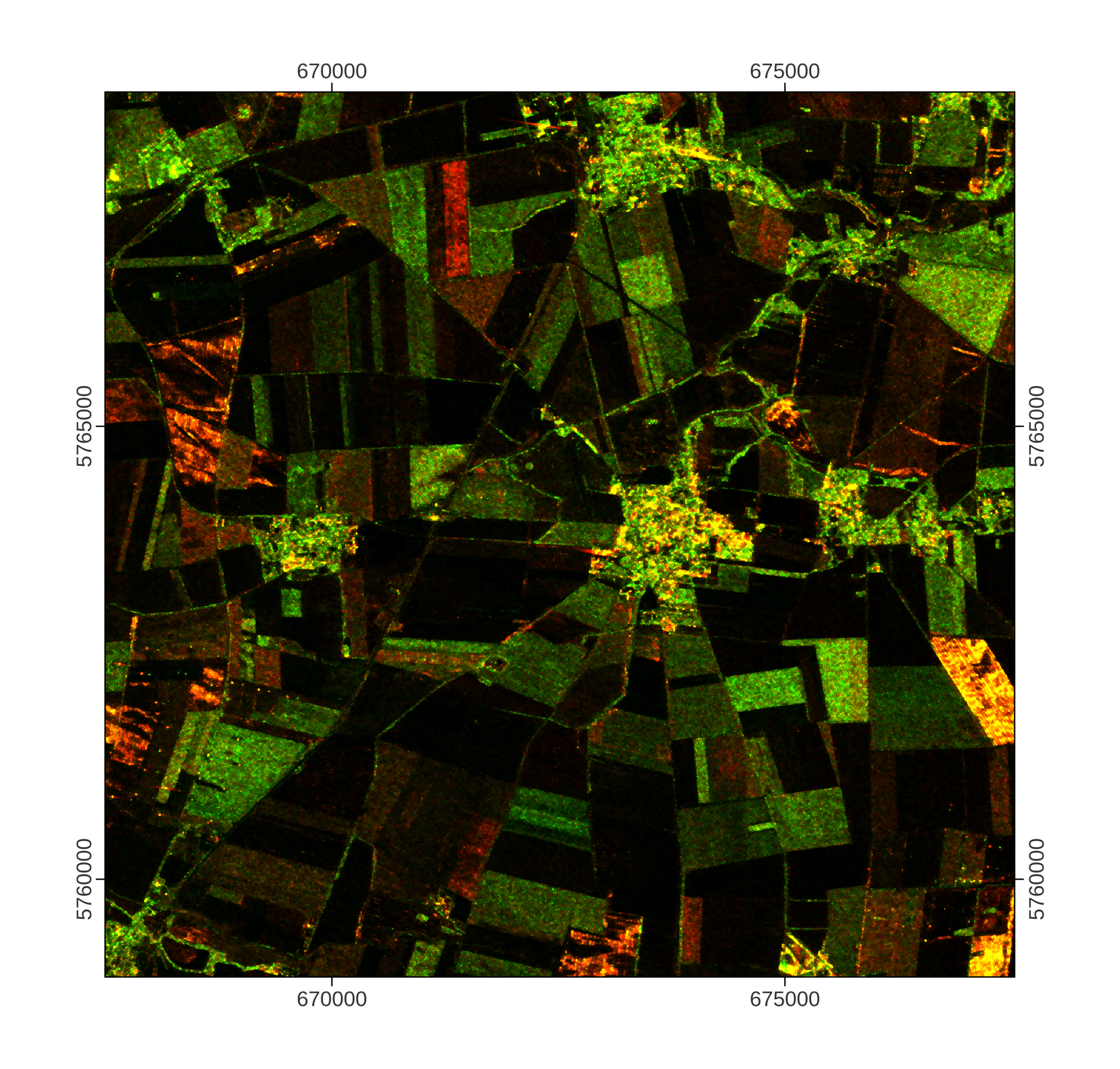
Figure 22: Gamma0 backscatter within subset of 32UPC tile on 18th of July 2024. Coordinate System: WGS 1984 UTM Zone 32N. Red – VV, green – VH.
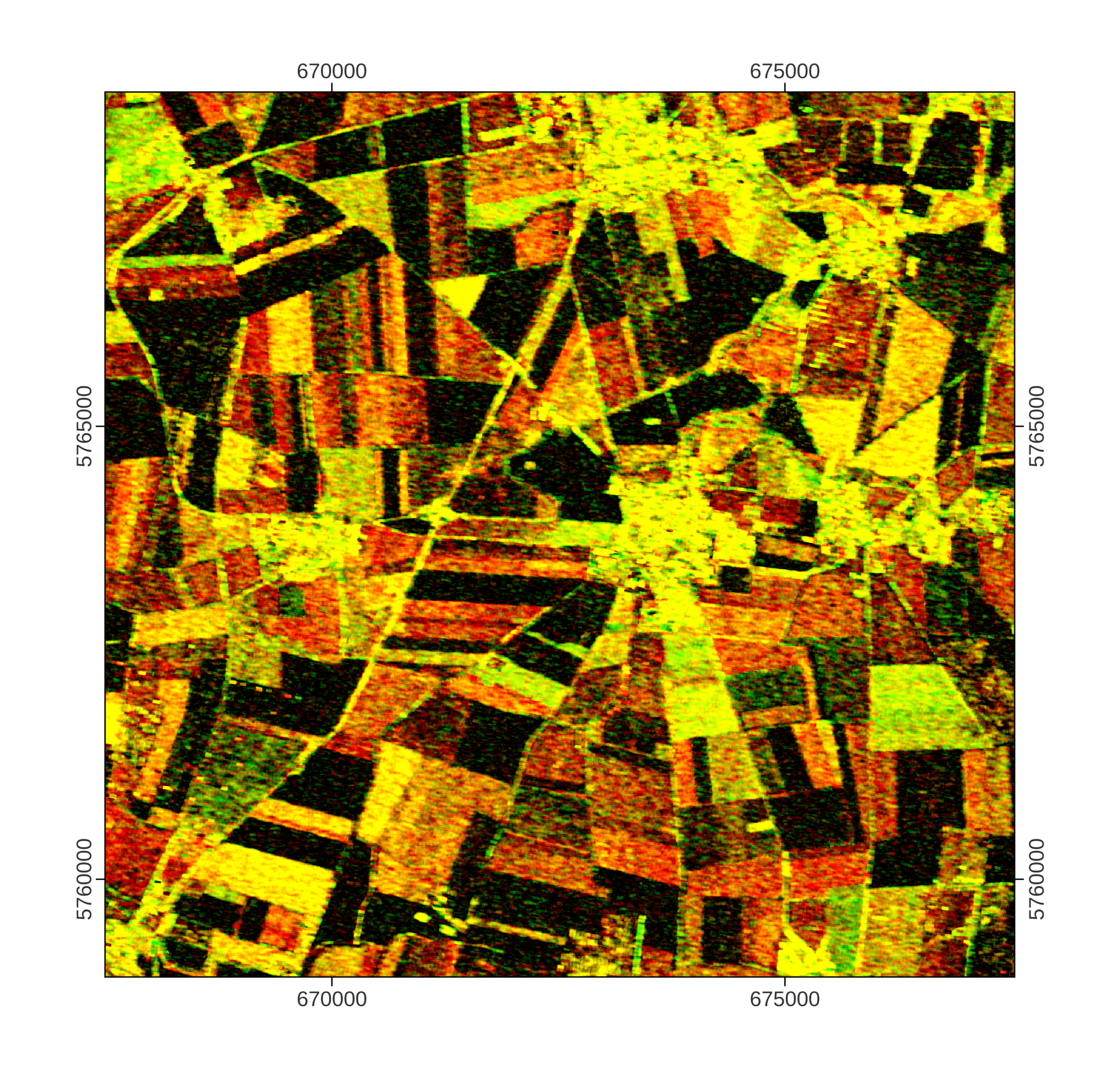
Figure 23: Coherence within subset of 32UPC tile on 2nd – 18th of July 2024. Coordinate System: WGS 1984 UTM Zone 32N. Red – VV, green – VH.
4. Conclusions
Representative datasets for the upcoming Copernicus Sentinel Expansion Missions CHIME, LSTM and ROSE-L were generated for three test-sites and two vegetation seasons. As a result, realistic time series for the years 2024 and 2025 were derived from existing sensor data and provided for regions in Germany, Belgium, and Estonia. They are publicly accessible to any interested user in three different collections within the ESA Project Results Repository (VISTA, 2026; VITO, 2026; KappaZeta, 2026).
The main focus of the datasets is the vegetated area, especially the agricultural areas. Nevertheless, complete spatial datasets covering all land uses were derived to make sure that as many users as possible could benefit from the datasets. Validation results indicate that the proposed simulation framework can generate spectrally and spatially consistent scenes. For CHIME-like data, high correlation coefficients, low SID values, and moderate SAM values across all validated scenes demonstrate that the simulated data preserve spectral shape and relative radiometric behavior despite being derived from multispectral Sentinel-2 inputs. For LSTM-like data, cross-calibration with ECOSTRESS data was not necessary, so that the ECOSTRESS data could be utilized directly as validation data, showing high correlations. For ROSE-L-like data, computed backscatter and coherence values remain within the nominal range and visual inspection shows no abnormalities in the results.
Thus, representative datasets of these three future sensors are now available which allow the development of innovative products which synergistically use high-resolution hyperspectral, thermal and L-band radar data is thus made possible. This enables rapid data exploitation as soon as real data from the Copernicus Sentinel Expansion Missions becomes available.
Appendix A: Additional Validation Results
A.1. Validation of CHIME data from 13.05.2024 by EnMAP data from 14.05.2024 in AOI 32UPC
A.1.1. Scene Pair 1
Per-band Metrics:
Pixel-wise Spectral Correlation:
A.1.2. Scene Pair 2
Per-band Metrics:
Pixel-wise Spectral Correlation:
A.1.3. Scene Pair 3
Per-band Metrics
Pixel-wise Spectral Correlation
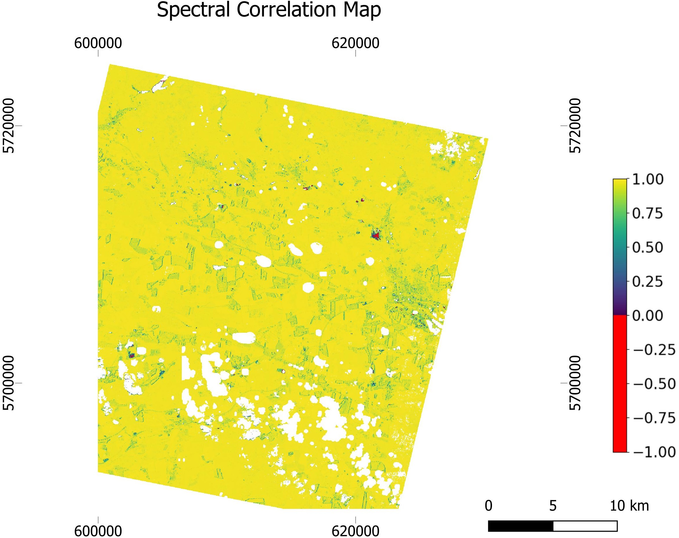
A.2. Validation of CHIME data from 29.07.2024 by EnMAP data from 30.07.2024 in AOI 32UPC
A.2.1. Scene Pair 4
Per-band Metrics
Pixel-wise Spectral Correlation
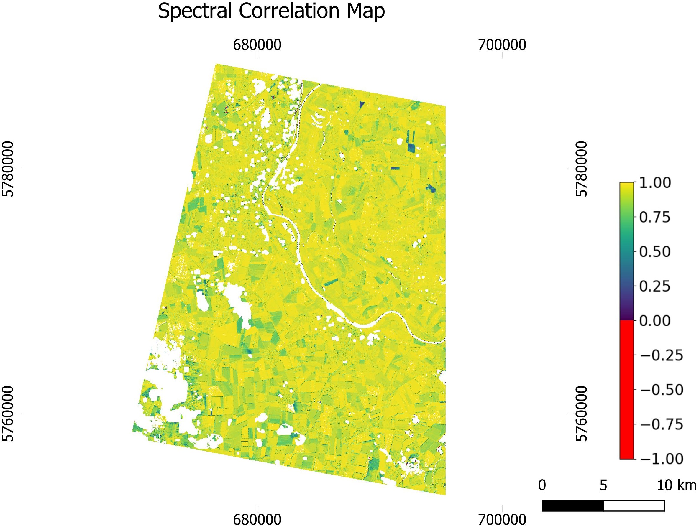
A.2.2. Scene Pair 5
Per-band Metrics
Pixel-wise Spectral Correlation
Author Contributions
Conceptualization: Silke Migdall, Heike Bach
Methodology: Silke Migdall, Heike Bach, Sandra Dotzler, Astrid Vannoppen, Louis Snyders, Joris Blommaert, Mihkel Veske, Tanel Tamm, Catherine Akinyi Odera
Software: Anusha Sanmathi Sathyaniranjan
Validation: Anusha Sanmathi Sathyaniranjan, Sandra Dotzler, Astrid Vannoppen, Louis Snyders, Mihkel Veske
Formal analysis: Anusha Sanmathi Sathyaniranjan, Sandra Dotzler, Christian Miesgang, Astrid Vannoppen, Louis Snyders, Mihkel Veske, Tetiana Shtym
Investigation: Sandra Dotzler, Christian Miesgang, Mihkel Veske, Tetiana Shtym, Catherine Akinyi Odera
Resources: Heike Bach
Data Curation: Christian Miesgang, Astrid Vannoppen, Louis Snyders, Mihkel Veske, Sven Kautlenbach, Tanel Tamm
Writing – Original Draft: Christian Miesgang, Sandra Dotzler, Anusha Sanmathi Sathyaniranjan, Silke Migdall, Astrid Vannoppen, Louis Snyders, Mihkel Veske, Catherine Akinyi Odera
Writing – Review & Editing: Christian Miesgang, Silke Migdall, Heike Bach, Sandra Dotzler, Astrid Vannoppen, Louis Snyders, Joris Blommaert, Mihkel Veske, Catherine Akinyi Odera
Visualization: Christian Miesgang, Sandra Dotzler, Anusha Sanmathi Sathyaniranjan, Silke Migdall, Astrid Vannoppen, Louis Snyders, Mihkel Veske
Supervision: Silke Migdall, Christian Miesgang, Joris Blommaert, Catherine Akinyi Odera
Project administration: Christian Miesgang, Silke Migdall, Joris Blommaert, Catherine Akinyi Odera
Funding acquisition: Silke Migdall, Heike Bach, Joris Blommaert, Tanel Tamm
Declaration of competing interest
The authors declare that they have no known competing financial interests or personal relationships that could have appeared to influence the work reported in this paper.
Acknowledgements
The contributions of EurA AG, specifically Johannes Schmidt and Mauricio Chaves-Vargas, to the study are explicitly acknowledged. Additionally, the authors thank the study’s Champion Users Pfeifer & Langen, Männiku Teravili and Aaspero Agro.
Funding
The work presented here has been funded by ESA in the Sentinel Users Preparation (SUP) Initiative under ESA Contract No. 4000145754/24/I-DT-bgh.
References
Bach, H., Verhoef, W. (2002). Simulation of SPECTRA like scenes using coupled leaf, canopy and atmospheric radiative transfer models. Recent Advances in Quantitative Remote Sensing, (ed. J. Sobrino), 863-870.
Baldridge, A. M., Hook S.J., Grove C.I., Rivera G. (2009). The ASTER Spectral Library Version 2.0. Remote Sensing of Environment, 113, 711-715 DOI: 10.1016/j.rse.2008.11.007.
Chang, C.-I. (2000). An information-theoretic approach to spectral variability, similarity, and discrimination for hyperspectral image analysis. IEEE Transactions on Information Theory, 46(5), 1927–1932, DOI: 10.1109/18.857802.
Copernicus (2024). OBSERVER: Advancing Earth Observation with the Copernicus Sentinel Expansion Missions. URL: https://www.copernicus.eu/en/news/news/observer-advancing-earth-observation-copernicus-sentinel-expansion-missions (accessed March 4, 2026).
Chabrillat, S., Foerster, S., Segl, K., Beamish, A., Brell, M., Asadzadeh, S., Milewski, R., Ward, K.J., Brosinsky, A., Koch, K., Scheffler, D., Guillaso, S., Kokhanovsky, A., Roessner, S., Guanter, L., Kaufmann, H., Pinnel, N., Carmona, E., Storch, T., Hank, T., Berger, K., Wocher, M., Hostert, P., van der Linden, S., Okujeni, A., Janz, A., Jakimow, B., Bracher, A., Soppa, M.A., Alvarado, L.M.A., Buddenbaum,H., Heim, B., Heiden, U., Moreno, J., Ong, C., Bohn, N., Green, R.O., Bachmann, M., Kokaly, R., Schodlok, M., Painter, T.H., Gascon, F., Buongiorno, F., Mottus, M., Brando, V.E., Feilhauer, H., Betz, M., Baur, S., Feckl, R., Schickling, A., Krieger, V., Bock, M., La Porta, L., Fischer, S. (2024). The EnMAP spaceborne imaging spectroscopy mission: Initial scientific results two years after launch. Remote Sensing of Environment, 315, 114379. DOI: 10.1016/j.rse.2024.114379.
DHI GRAS. (2020). User Manual for Sen-ET Snap Plugin (V1.1.0). URL: https://www.esa-sen4et.org/static/media/sen-et-user-manual-v1.1.0.2cd617fb322658397542.pdf.
Esri (2017). World Imagery. ArcGIS Online. URL: https://www.arcgis.com/home/item.html?id=974d45be315c4c87b2ac32be59af9a0b (accessed June 18, 2026).
Gao, F., Kustas, W. P., Anderson, M. C. (2012). A Data Mining Approach for Sharpening Thermal Satellite Imagery over Land. Remote Sensing, 4(11), 3287–3319. DOI: 10.3390/RS4113287.
Guzinski, R., Nieto, H., Sandholt, I., Karamitilios, G. (2020). Modelling High-Resolution Actual Evapotranspiration through Sentinel-2 and Sentinel-3 Data Fusion. Remote Sensing, 12(9), 1433. DOI: 10.3390/RS12091433.
KappaZeta (2026). ROSE-L representative dataset (CHILL-Y). URL: https://browser.apex.esa.int/external/eoresults.esa.int/stac/collections/roseL_rep_dataset?.language=de (accessed April 15, 2026).
Koetz, B., Baschek, B., Bastiaanssen, W., Berger, M., Blommaert, J., Alamanac, A. B., Barat, I., Fabrizia Buongiorno, M., D’andrimont, R., Bello, U. Del, Drusch, M., Duca, R., Gamet, P., Gascon, F., Ghent, D., Guzinski, R., Hoogeveen, J., Hook, S., Manolis, I., Udelhofen, T. (2021). Copernicus High Spatio-Temporal Resolution Land Surface Temperature Mission: Mission Requirements Document. URL: https://sentiwiki.copernicus.eu/__attachments/1678167/ESA-EOPSM-HSTR-MRD-3276%20-%20Copernicus%20High%20Spatio-Temporal%20Resolution%20Land%20Surface%20Temperature%20Mission%202021%20-%203.0.pdf?inst-v=5f22af6a-d79a-4a5b-a820-1fdb4aabe8f4.
Kruse, F. A., Lefkoff, A. B., Boardman, J. W., Heidebrecht, K. B., Shapiro, A. T., Barloon, P. J., Goetz, A. F. H., (1993). The Spectral Image Processing System (SIPS)—Interactive visualization and analysis of imaging spectrometer data. Remote Sensing of Environment, 44(2–3), 145–163, DOI: 10.1016/0034-4257(93)90013-N.
Meerdink, S. K., Hook, S. J., Roberts, D. A., Abbott, E. A. (2019). The ECOSTRESS spectral library version 1.0. Remote Sensing of Environment, 230(111196), 1–8, DOI: 10.1016/j.rse.2019.05.015.
Migdall, S., Bach, H., Kaufmann, H. (2010). Simulation of EnMAP-like hyperspectral images based on textural information and a radiative transfer approach. In Proceedings of the Hyperspectral Workshop 2010, European Space Agency (ESA), Frascati, Italy. URL: https://earth.esa.int/documents/20142/37627/Hyperspectral+Workshop+2010.pdf/a2da4d2d-4858-1ceb-6aa4-b7289d350033?t=1703155366512.
Rast, M., Adams, J., Gascon, F., Nieke, J., Ananasso, C., Bach, H., Ben Dor, E., Chabrillat, S., Colombo, R., Feret, J.-B., Giardino, C., Green, R. O., Guanter, L., Marsh, S., Ong, C., Rum, G., Schaepman, M., Schlerf, M., Schodlok, M., Skidmore, A. K., Storch, T., Strobl, P., Williams, M. (2021). Copernicus Hyperspectral Imaging Mission for the Environment – Mission Requirements Document. Issue 3.0. Issue Date 21/01/2021. URL: https://esamultimedia.esa.int/docs/EarthObservation/Copernicus_CHIME_MRD_v3.0_Issued_21_01_2021.pdf.
Revel, C., Lonjou, V., Marcq S., Desjardins C., Fougnie B., Coppolani-Delle Luche C., Guilleminot N., Lacamp A.-S., Lourme E., Miquel C., Lenot, X. (2019). Sentinel-2A and 2B Absolute Calibration Monitoring. European Journal of Remote Sensing, 52(1), 122–137. DOI: 10.1080/22797254.2018.1562311.
Sandvik, B. (2008). TM_WORLD_BORDERS-0.3 [ shapefile dataset ]. Thematic Mapping. URL: http://thematicmapping.org/downloads/world_borders.php.
Schickling A., Chabrillat S., Storch T., Fischer S. (2021). EnMAP: THE GERMAN SPACEBORNE IMAGING SPECTROSCOPY MISSION. OSA Optical Sensors and Sensing Congress 2021 (AIS, FTS, HISE, SENSORS, ES). DOI: 10.1364/HISE.2021.HF4E.1.
Small, D. (2011). Flattening gamma: Radiometric terrain correction for SAR imagery. IEEE Transactions on Geoscience and Remote Sensing, 49(8), 3081-3093. DOI: 10.1109/TGRS.2011.2120616.
SNAP (2025). ESA Sentinel Application Platform v11.0.1. URL: http://step.esa.int (accessed August 29, 2025).
Snyders L, Blommaert J, León-Tavares J, Degerickx J (2025). Identification, Characterization and Correction of Directional Anisotropy in High-Resolution Land Surface Temperature through a Comparison of Sharpened Sentinel-3 with ECOSTRESS Data. Recent Advances in Remote Sensing, 2025, 2 (8). DOI: 10.62880/rars25008.
Stuffler T., Kaufmann C., Hofer S., Förster K.P., Schreier G., Mueller A., Eckardt A., Bach H., Penné B., Benz U., Haydn R. (2007). The EnMAP hyperspectral imager – An advanced optical payload for future applications in Earth observation programmes. Acta Astronautica, 61 (1–6), 2007, 115-120. DOI: 10.1016/j.actaastro.2007.01.033. van der Meer, F. (2006). The effectiveness of spectral similarity measures for the analysis of hyperspectral imagery. International Journal of Applied Earth Observation and Geoinformation, 8(1), 3–17. DOI: 10.1016/j.jag.2005.06.001.
Verhoef, W., Bach, H., (2007). Coupled soil–leaf-canopy and atmosphere radiative transfer modeling to simulate hyperspectral multi-angular surface reflectance and TOA radiance data. Remote Sensing of Environment, 109(2), 166-182. DOI: 10.1016/j.rse.2006.12.013.
Verhoef, W., Bach, H. (2012). Simulation of Sentinel-3 images by four stream surface atmosphere radiative transfer modeling in the optical and thermal domains. Remote sensing of Environment, 120, 197-207. DOI: 10.1016/j.rse.2011.10.034.
VISTA (2026). CHIME representative dataset (CHILL-Y). URL: https://browser.apex.esa.int/external/eoresults.esa.int/stac/collections/CHIME_rep_dataset?.language=de (accessed April 15, 2026).
VITO (2026). LSTM-like Land Surface Temperature (CHILL-Y). URL: https://browser.apex.esa.int/external/eoresults.esa.int/stac/collections/chilly-lstm-like-lst?.language=de (accessed April 15, 2026).
Wang, Z., Bovik, A. C., Sheikh, H. R., Simoncelli, E. P., (2004). Image quality assessment: From error visibility to structural similarity. IEEE Transactions on Image Processing, 13(4), 600–612. DOI: 10.1109/TIP.2003.819861.
Publisher’s Note
The statements, opinions and data contained in all publications are solely those of the individual author(s) and contributor(s) and not of Recent Advances S.L. and/or the editor(s). Recent Advances S.L. and/or the editor(s) disclaim responsability for any injury to people or property resulting from any ideas, methods, instructions or products referred to in the content.