



Identification, Characterization and Correction of Directional Anisotropy in High-Resolution Land Surface Temperature through a Comparison of Sharpened Sentinel-3 with ECOSTRESS Data
Louis Snyders
1,2*,Joris Blommaert

1,2, Jonathan León-Tavares
1, Jeroen Degerickx
1- VITO, 2400 Mol, Belgium.
- Department of Physics, Vrije Universiteit Brussel, 1050 Elsene, Belgium.
* Author to whom correspondence should be addressed.

Abstract
This study identifies, characterizes and corrects for directional effects in high-resolution (HR) Land Surface Temperature (LST) maps based on a comparison of sharpened Sentinel-3 (S3) and ECOSTRESS data at 70-meter resolution. Firstly, the two HR LST datasets were assembled. A Data Mining Sharpener (DMS) derived HR LST to overcome the lack of HR data. This technique sharpened 1 kilometer spatial resolution LST from the S3 Sea and Land Surface Temperature Radiometer (SLSTR), for the Flanders region from 2019 to 2024. The DMS uses a bagging ensemble, that incorporates Sentinel- 2 (S2) Multi-Spectral Instrument (MSI) reflectance bands and Copernicus Digital Elevation Model (DEM) data, to enhance the spatial resolution of S3 SLSTR LST. Quasi-simultaneous ECOSTRESS LST acquisitions, for the same region, were acquired to serve as a secondary data source. Secondly, the combined dataset, containing multi-angular observation pairs, was used for analysing directional effects. After cross-calibrating the observation pairs, directional effects are identified through pixel-by-pixel comparisons. A Vinnikov-Roujean-Lagouarde (RL) parametric model simulated directional effects up to 1.6 K. Additionally, case-specific parametric models have been established, characterizing specific morning, night, seasonal, land cover and vegetation density effects. A validation study demonstrates that the proposed correction methodology decreases LST differences of the observation pairs, with tailored strategies for specific conditions yielding the best results. Our study underscores the importance of considering directional effects in HR LST retrievals and provides a global correction framework for upcoming HR thermal missions, including LSTM, TRISHNA and SBG.Keywords
Land Surface Temperature, Directional Anisotropy, Sentinel-3, ECOSTRESS, Data Mining Sharpener1. Introduction
Thermal infrared (TIR) remote sensing has emerged as a powerful tool for generating time series of land surface temperature (LST) data at both global and local scales. TIR sensors measure the radiation emitted by the Earth’s surface in the 8–12μm range, which is directly related to the surface temperature. This capability is valuable for monitoring applications in various domains, including natural hazards, urban heat islands, water management, among others (Sobrino et al., 2016). Specifically, LST can assist in detecting wildfires (Vlassova et al., 2014) , volcanic activity (Cigna et al., 2020), air pollution (Feizizadeh and Blaschke, 2013) and oil spills (Casciello et al., 2011), urban planning (Coutts et al., 2016) and water management activities. Within the water management domain, regular LST observations are key for evapotranspiration (ET) estimation and drought monitoring (González-Dugo et al., 2006; Zarco-Tejada et al., 2013), where timely and accurate LST information, within 1 K (Sobrino et al., 2016), is required for mitigating the adverse impacts on agriculture and ecosystems. Common LST retrieval algorithms are the Split-Window (SW) algorithm, used for Sentinel-3 (Zheng et al., 2019), MODIS (Wang et al., 2019) and Landsat (Rozenstein et al., 2014), and the Temperature and Emissivity Separation (TES) algorithm, used for ECOsystem Spaceborne Thermal Radiometer Experiment on Space Station (ECOSTRESS) (Hulley and Hook, 2018). The SW method is based on the difference in brightness temperatures, derived from thermal radiation, measured in two or more adjacent thermal infrared bands to correct for atmospheric effects and retrieve LST (Wan and Dozier, 1996). The TES method simultaneously retrieves LST and Land Surface Emissivity (LSE) through iteratively separating both quantities using data from multiple TIR bands (Gillespie et al., 1998).
Thus far, thermal remote sensing has received far less attention compared to optical remote sensing due to the lack of high spatio-temporal TIR datasets (Neinavaz et al., 2021). Current TIR products often compromise between spatial and temporal resolution (Gerhards et al., 2019), which limits their applicability for precision agriculture and drought monitoring at field scale (Sobrino et al., 2016). Despite Landsat 8 and 9 offering a sufficient thermal resolution of 100 m (Mahlein, 2016), the combined revisit time of eight to sixteen days is insufficient to detect rapid changes in surface moisture or crop phenology, especially in areas with persistent cloud cover. Other current thermal infrared sensing satellites offer high temporal resolution(e.g., MODIS, AVHRR, VIIRS, Sentinel-3) but coarse spatial resolution (1 km). The next generation of satellite platforms with high-resolution (HR) thermal capabilities, including the Land Surface Temperature Monitoring (LSTM) (Koetz et al., 2018), the Thermal Infra-Red Imaging Satellite for High-resolution Natural Resource Assessment (TRISHNA) (Roujean et al., 2021), and the Surface Biology and Geology (SBG) (Stavros et al., 2023), will effectively tackle the current lack of high spatio-temporal TIR capabilities and aims to provide daily field-scale LST, offering promising perspectives for the use of TIR for the (early) detection of crop water stress from space. Multi-sensor scaling techniques, such as pan-sharpening or thermal sharpening, aim to mitigate the issue of lacking high tempo-spatial resolution LST through spatial enhancement of available low-resolution LST products (Gerhards et al., 2019). Thermal sharpening involves modelling the relationship between optical and thermal data at coarse spatial resolution and applying it to HR optical data to produce HR thermal imagery. Techniques like TsHARP use fractional vegetation cover (fc) as an explanatory variable for thermal behaviour (Agam et al., 2007; Kustas et al., 2003), but are inconsistent across landscapes due to the variability in the relationship between LST and fc, which can differ significantly based on vegetation type, soil conditions and climate (Chen et al., 2011; Jeganathan et al., 2011). Gao et al. (2012) introduced a data mining sharpener (DMS) to sharpen LST, outperforming traditional methods, especially in heterogeneous landscapes. The European Space Agency (ESA) Sentinels for Evapotranspiration (Sen-ET) project adopted the DMS to produce HR ET estimates based on Sentinel-2 (S2) surface reflectance and Sentinel-3 (S3) LST (Guzinski et al., 2020).
Current low-resolution TIR satellites, such as MODIS, VIIRS, S3 have swath widths of 2330 km (Masuoka et al., 2002), 3060 km (Cao et al., 2017) and 1420 km (Cornara et al., 2017), respectively, necessary for large coverage. Due to the large field of views and scan angles, the viewing geometry and the solar angles change substantially from observation to observation. However, acquired LST is the result of the ensemble of radiance from scene elements and thus varies with the observed element proportions within a pixel (Li et al., 2013). These directional effects, influencing LST, comprises the gap and the hotspot effect. The gap effect is the result of the gap fraction (Nilson,1999), which causes the observer to retrieve temperatures from different scene element materials, each with a specific temperature and emissivity, whichchanges with viewing angle, under the same illumination conditions. As a result, TIR measurements over crop fields will deliver high temperatures if obtained close to the nadir position, due to the higher fraction of observed hot soil, as opposed to low temperatures for elevated viewing angles, due to the increased observed fraction of the colder canopy. The hotspot effect, on the other hand, depends on the illumination conditions and is the result of the ensemble of observed sunlit and shaded scene elements and thus depends both on the viewing angles and solar angles (Jupp and Strahler, 1991). Directional effects, firstly identified in 1962 (Monteith and Szeicz, 1962), is often referred to as directional anisotropy (DA) or thermal radiation directionality (TRD), and can result in temperature differences up to 11 K for modelled agricultural fields on a summer day (Duffour et al., 2016a), up to 14 K over urban areas (Lagouarde et al., 2010), or for in-field observations even up to 16 K (Kimes and Kirchner, 1983). Furthermore, Duffour et al. (2016b) showed that, based on Radiative Transfer Modelling (RTM), DA depends on seasonal trends and geometrical structure, such as Leaf Area Index (LAI), of the canopy. Correcting for these directional effects is essential to ensure high
consistency and reliability of the data. The development of parametric models in the form of semi-empirical thermal infrared kernel-driven models (KDMs) addresses these directional effects, by modelling the expected LST as function of the viewing and solar geometry, based on simple gap and hotspot functions. These models, which only require the determination of a handful of parameter coefficients, offer a promising solution, being a trade-off between operability and accuracy, towards an operational correction of directional effects (Cao et al., 2019, 2021).
A multitude of three-parameter KDMs exists. Originally, KDMs were extracted from the visible and near-infrared (VNIR) bidirectional reflectance distribution function (BRDF) (Liang and Strahler, 1994) and directly used in the TIR domain to model the TRD. The Roujean-Lagouarde (RL) model, a hotspot model, was tested for HR airborne TIR measurements over Toulouse (Lagouarde and Irvine, 2008), and for a vegetation scene and scope simulations (Duffour et al., 2016b). The Ross-Li model was tested using airborne images and 4SAIL simulations (Hu et al., 2016). Additional models emerged, specifically designed for TIR radiation, such as the LSF-Li model (Su et al., 2002) and Vinnikov model, which was applied to lowresolution GOES acquisitions (Vinnikov et al., 2012) and MODIS and TERRA acquisitions (Ermida et al., 2017). Validation studies (Cao et al., 2019; Liu et al., 2018) showed the LSF-Li model outperformed others, with RL and Vinnikov models inadequate for non-hotspot and hotspot effects, respectively. By combining multiple kernels into a four-parameter KDM, such as Vinnikov-RL, accounting for non-hotspot and hotspot effects, respectively, the modelling
accuracy increases (Ermida et al., 2018). Building on this idea, (Cao et al., 2021) proposed the general framework for TIR kernel-driven modelling. The semi-empirical modelling framework, focused on the TIR region, capturesthe two main TRD effects, i.e., the non-hotspot effect or gap effect and the hotspot effect, by combining an isotropic, a gap and a hotspot kernel. The new framework allows for the combination of gap kernels with hotspot kernels, and all combinations can simulate continuous and discrete scenes with high accuracy.
This research aims to address directional effects in HR LST by combining thermal sharpening with a directional correction. This approach offers the potential to identify and characterize directional anisotropy in HR TIR data. Daily observations ensure sufficient data collection, while the sharpening technique provides field-scale resolution. The methodology overcomes the lack of HR LST datasets for researching directional effects. The characterization of these effects includes modelling directional effects for day, night, summer and winter observations, different land covers and varying canopy density through LAI. Additionally, the combination of thermal sharpening and DA modelling offers the opportunity to develop a directional correction to achieve daily HR LST and derived products, with minimized directional effects. Furthermore, the implementation of a directional correction within a thermal sharpening process provides a showcase for future HR thermal satellite missions, e.g. LSTM, TRISHNA and SBG, demonstrating the feasibility and benefits of directionally corrected HR thermal data for various applications. The primary objective of these missions is the monitoring of ET at field scale, which stresses the need for a directional correction to retrieve accurate LST retrievals, within 1 K, since it is the among the most significant parameters to estimate ET (Ambas and Baltas, 2012; Jiang et al., 2022; Taheri et al., 2022).
This study focuses on the following research objectives:
1.-Identification of directional effects in sharpened LST images.
2.-Characterization of directional effects in sharpened LST images.
3.-Development and cross-validation of a directional correction methodology for sharpened thermal data.
By addressing these objectives, this research aims to contribute to the field of thermal remote sensing by exposing the influence of directional effects in sharpened LST and showcasing the potential of a correction strategy for upcoming HR thermal missions. The structure of the paper is as follows: Section 2 Materials and Methods describes the thermal sharpening process based on the DMS, which fuses data from Sentinel-2 and Sentinel-3, for the study area, Flanders, covering the period from 2019 to 2024. Furthermore, it describes the cross-calibration and directional corrections achieved by comparing with the thermally sharpened Sentinel-3 data with ECOSTRESS data, along with the validation procedure. Section 3 presents the identified directional effects and corresponding models, in general and for specific cases, and the cross-validation of the directional correction. Section 4 elaborates on these results and Section 5 summarizes the key findings and the implications of the research.
2. Materials and Methods
The identification of directional effects required multi-angular acquisitions. This paper opted for the acquisition of multi-angular LST on a pixel level, by comparing sharpened S3 data, resulting from fusing S3, S2 and Digital Elevation Model (DEM) data, with ECOSTRESS data. As a result, each pixel corresponds to two acquisitions with different viewing angles. The benefit of this strategy is the possibility to characterize each pixel by land cover and LAI. After characterization, directional models can be constructed for various land covers and ranges of vegetation density. An alternative approach to obtain multi-angular LST is to compare all pixel temperatures within one acquisition since each pixel within that acquisition has a different acquisition angle (Michel et al., 2023). However, for satellite imagery, this approach has the disadvantage that large areas need to be considered to obtain a sufficiently large range of viewing angles. In such case, surface temperature trends might be mistaken for directional effects. For example, an acquisition of a coastal area during summer will return lower temperatures closer to the sea than for inland pixels. In such cases, assessing the temperature trend in the acquisition solely to directional effects is false.
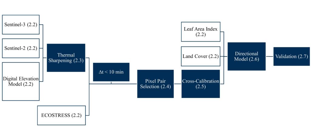
Figure 1: Overview of the research methodology with input data in white boxes and methodology steps in shaded boxes. The numbers in the boxes refer to the corresponding subsections.
Figure 1 provides an overview of the proposed methodology. A valid intercomparison of satellite data required similar conditions for S3 and ECOSTRESS observations. Therefore, simultaneous observations were vital to avoid the introduction of temporal discrepancies. However, perfect simultaneous observations were not achievable. Hence, an assumption arose: within a specific timeframe, temperature changes are negligible. Based on existing guidelines on LST validation and intercomparison, only S3 and ECOSTRESS observations were selected if they were acquired within a 10- minute timeframe (Guillevic et al., 2018).
The resulting acquisitions contained a large pixel pair data pool, which was further screened to select the best pixel pairs for cross-calibration of the two data sets and construction of directional models. First, a general directional model was created based on the resulting data pool. Additionally, case specific models were created based on extracted pixel pairs corresponding to morning, evening, summer and winter observations, and for specific land covers and LAI ranges.
2. 1 Region of Interest
To identify and characterize directional effects and validate the correction methodology, observations acquired during the six-year period from 2019 to 2024 were selected for three tiles from the S2 Universal Transverse Mercator (UTM) tiling grid: 31UDS, 31UES, and 31UFS. These tiles, each spanning 100 × 100 km2, correspond to the Flemish region (Belgium) and its surroundings. The region was chosen for several reasons. Firstly, Flanders is predominantly a plain with minimal elevation changes, which facilitated the identification and characterization of directional effects without the need to account for topographical variations. Secondly, the three tiles encompass a variety of land covers, including significant areas of water, urbanization, trees, and fields. Thirdly, Flanders’ latitude aligns with the 51.6◦ inclination angle of the ECOSTRESS-carrying orbiter, the International Space Station (ISS). Thus, Flanders’ latitude corresponds to the highest revisit times. Unlike the sun-synchronous orbits of S2 and S3, the ECOSTRESS orbit provides images of the region of interest (ROI) at various times of the day for each acquisition. Therefore, selecting an ROI with a high revisit time increased the number of observations and thus the potential availability of quasi-simultaneous observations with S3.
2.2. Input Data
Table 1 provides an overview of the used datasets. The following subsections elaborate on the specific datasets.
Table 1.-Datasets, sources, products, and remarks used in the study.

2.2.1 ECOSTRESS
ECOSTRESS (Fisher et al., 2020) data was acquired from the NASA Earthdata platform and included two files per acquisition: ECO1BGEO and ECO2LSTE. The ECO2LSTE version 1 data product (Hulley and Hook, 2018) contained atmospherically corrected LST and emissivity (LSTE) derived using the Temperature and Emissivity Separation (TES) algorithm based on five TIR bands. The data product, in the form of swath data with a spatial resolution of 70 m, contained multiple layers, including LST, Quality Control (QC), LST error, individual band emissivity and individual band emissivity error. A validation study showed a Root Mean Squared Error (RMSE) of 1.07 K and a Mean Absolute Error (MAE) of 0.40 K, and a cold bias of 0.75 K for temperatures below 295 K (Hulley et al., 2021). ECO1BGEO (Smyth and Leprince, 2018) contained geometric information, including height, land fraction, latitude, longitude, viewing zenith angle (VZA), viewing azimuth angle (VAA), solar zenith angle (SZA), solar azimuth angle (SAA), necessary for georeferencing the LST and extracting viewing geometry for identifying directional effects. Observations characterized by significant geolocation errors, identified by a False value for the metadata field “L1GEOMetadata/OrbitCorrectionPerformed”, were discarded from our analysis. Additionally, the QC layer, from ECO2LSTE, was used to mask the LST to select only the best quality pixels, by only considering pixels corresponding to QC bits 1&0 being equal to 00 (Hulley and Hook, 2018). As a result, cloud-affected pixels, pixels falling on missing scan lines, or pixels suffering from low transmissivity were removed.
2.2.2. Data Copernicus Data for Retrieval of Sharpened Sentinel-3 LST
The sharpening algorithm relied on Copernicus data: Sentinel-2 Multi-Spectral Instrument (MSI) optical data, Sentinel-3 SLSTR thermal data, and the 30 m Copernicus Digital Elevation Model (DEM). The required input data were retrieved from the Copernicus Data Space Ecosystem, through VITO’s Terrascope service (https://terrascope.be). The S3 data included data resulting from both Sentinel-3A, launched in 2016, and Sentinel-3B, launched in 2018, which have identical orbits but a phase shift of 140◦. Each satellite platform contained four main instruments, including the Sea and Land Surface Temperature Radiometer (SLSTR) (Koetz et al., 2021) providing observations from eleven spectral bands. LST was derived based on applying the Split-Window (SW) algorithm to the two available TIR bands (Ghent et al., 2021). The final level-2 LST data, which was provided in multiple files, included the key datafile, LST_in.nc, containing LST and LST_uncertainty, a geometry file with satellite and solar angles,geometry_tn.nc, and a cloud masking file, flags_in.nc, among other files. The layers of interest, LST, LST_uncertainty, Vza, Vaa, Sza, Saa, MSK, were retrieved by using the Sentinel Applications Platform (SNAP) tool. Table 5 in Appendix A provides details on the parameters in the .xml file used to download the S3 data. The SW algorithm was expected to achieve 1 − 3 K accuracies, with the best accuracies for night observations, due to absent differential surface heating (Ghent et al., 2021). A validation study showed uncertainties of 1.3 K and 1.5 K for the operational LST product for Sentinel-3A SLSTR and Sentinel-3B SLSTR, respectively (Pérez-Planells et al., 2021). Furthermore, a hot bias was identified, which varies from an overestimation of 1.1 K to 1.9 K according to different studies (Sánchez et al., 2023). The S3 data is expected to contain more directional effects than ECOSTRESS since the S3 SLSTR instrument operates with a conical scanning mechanism at ±55◦, whereas the ECOSTRESS scanner is limited to ±25◦. The S3 orbit is a near-polar, sun-synchronous orbit with a descending node equatorial crossing at 10:00 mean local solar time. Due to the sunsynchronous orbit, the satellite passes over the same location at the same local solar time, ensuring consistent sun angles for each pass. However, the sun’s position changes throughout the year, resulting in variations in illumination angles over different seasons. Furthermore, every orbit provides night observations around 21 : 00 h mean local solar time. Since ECOSTRESS follows the ISS orbit, it randomly coincides with S3 observations. The original S3 data has a spatial resolution of 1 km, compared to the 70-meter resolution of ECOSTRESS. For a pixel based comparison of the two images, pixel alignment was necessary. Therefore, the S2 and DEM input layers, which determine the sharpening output resolution, were first resampled to match the corresponding ECOSTRESS LST map, using cubic spline as the resampling method. Based on the resulting inputs, sharpened S3 LST can be obtained.
2.2.3. Land Cover and Leaf Area Index
To investigate the directional effects of different land cover types, the WorldCover map was used, which provides global land cover products for 2020 (Zanaga et al., 2021) and 2021 (Zanaga et al., 2022) at 10 m resolution, available on the VITO Terrascope platform (https://terrascope.be). Validation reports have showed an overall accuracy for Europe of 76.8% and 77.9% for the 2020 and 2021 maps, respectively (Linlin et al., 2021; Panpan et al., 2022). Since there was no land cover map available for 2019, 2022, 2023, and 2024, the WorldCover maps of 2020 and 2021 were used to assign land covers to the 2019 observations and the 2022-2024 observations, respectively. We assumed that land cover did not change significantly between 2019 and 2020 and between 2021 and 2024. The analysis was restricted to land cover classes with sufficient pixel pairs: permanent water bodies, tree cover, grassland, cropland and built-up.
Since multiple 10 m land cover pixels fitted within the 70 m pixel pair, the mode of land cover pixels within the 70 m pixel was assigned to the pixel pair. Furthermore, a distinction was made between mixed and pure pixels after resampling. A pure pixel is a pixel resampled to 70 m for which all the underlying original 10 m land cover pixels belong to the same land cover class. Contrary, a mixed pixel is pixel resampled to 70 m for which the underlying pixels belong to at least two different land cover classes. Selecting pure pixels contributed to the accurate characterization of directional effects.
The characterization of directional effects for vegetation density was based on the Leaf Area Index (LAI), made available on VITO’s TerraScope platform (Piccard et al., 2020). Since LAI is available at 20 m, LAI, acquired within two days from the relevant LST macquisition, was resampled, using average resampling, to match the 70 m resolution of the sharpened S3 and ECOSTRESS grid. LAI was only considered for natural land covers: tree cover, shrubland, grassland, cropland, bare/sparse vegetation and herbaceous wetland. Through exclusion of the other categories, the total number of pixels evaluated for the LAI characterization was reduced.
2.3. Thermal Sharpening
The thermal sharpening method used in this study was based on the DMS using S2 reflectance bands and a DEM to predict S3 LST (Gao et al., 2012; Guzinski et al., 2020), and implemented by Guzinski (2017) in the pyDMS repository. The DMS assumes a relationship between thermal and optical features in Earth Observation (EO) data, leveraging an ensemble of decision trees through a bagging algorithm. This relationship is established initially at the native low S3 resolution and then applied to HR optical data to obtain sharpened thermal data.
In our study, each 1000 m resolution S3 acquisition was paired with a 10-day S2 composite at 20 m resolution. The S2 composite and DEM data were first resampled to match ECOSTRESS’s 70-meter resolution. A bagging algorithm fitted each composite S2-S3 scene pair to sharpen S3 LST from 1000 m to 70 m. A final bias correction ensured energy conservation between the original low-resolution (LR) and the generated HR LST maps. Table 6 in Appendix A provides an overview of parameters used in pyDMS. For more algorithm details, we refer to the Sen-ET algorithm manual (DHIGRASS, 2020).
We implemented three main adaptations in the sharpening algorithm. Firstly, our implementation of the algorithm used a 10-day composite for S2 instead of a single observation to minimize cloud cover and reduce noise. Secondly, we resampled our input data to the corresponding ECOSTRESS acquisition. Consequently, the final S3 LST product had a resolution of 70 meters. Thirdly, unlike the original Sen-ET implementation, the sharpener was trained only on the full Sentinel-2 tile, rather than using both the global and local moving window approaches.
The moving window approach was not applied because each S2 tile, covering an area of 110 km x 110 km, was sharpened. This would have led to a high computational cost for every single global model, that was constructed for each individual observation pair. Introducing additional local models with a large window size, for example, 37 km x 37 km would have increased the number of bagging models with a factor 10. While using smaller window sizes could better capture local regression, computational costs would have further increased. The global model has the disadvantage of not capturing the local spatial variability in the regression relationships. However, its large spatial extent offers the advantage of a broad and diverse training set for the bagging algorithm. We consider the approach as a practical compromise between computational efficiency and model performance.
The sharpening procedure introduces additional uncertainty, next to the uncertainty already present within the S3 LR LST. The resulting uncertainty in LSTS3HR for pixel i is:
where σLSTSLR, j is the uncertainty in the S3 LR LST of pixel j corresponding to the S3 HR LST of pixel i. Note that this means that the uncertainty is equal for all HR pixels that fall within the same LR pixel. Gao et al. (2012) assessed the uncertainty introduced by the sharpening by using HR Landsat LST as reference data and created low-resolution LST by aggregating the reference data. They sharpened the low-resolution LST with HR reflectance bands and compared it with reference data for three areas: rainfed agriculture, irrigated agriculture, and natural vegetation with complex terrain. The expected MAE for sharpening from 1000 m to 70 m, based on the provided MAE for Landsat at different sharpening ratios and linear interpolation of the documented sharpening ratios, is 0.65−1.20 K, 0.78 K and 2.04 K for the rainfed, irrigated and complex site, relatively. Therefore, in this paper we assume a sharpening uncertainty, σsharpening, of 2 K , representing the most challenging conditions and provide a conservative estimate. Additionally, the choice is supported by the fact that the region of interest in our study includes a mixture of landscapes. The resulting estimated uncertainty within LSTS3HR,i becomes:
2.4 Pixel Pair Selection
For computational efficiency, only ten percent of pixels per simultaneous acquisition pair, i.e. a S3 and ECOSTRESS observation acquired within a ten-minute timeframe, were randomly selected. To avoid comparing image pairs affected by misidentified clouds or significant shadowing, we removed observation pairs where the median ΔLST of pixel pairs deviated by more than 5 K from the overall median ΔLST of 1.2 K . Observation pairs with a median ΔLST outside the [-3.8 K, 6.2 K] range were considered corrupted as such median difference couldn’t be attributed to directional effects. While individual pixels can still exhibit higher temperature differences, it is unreasonable to assume that directional effects alone would cause such large deviations consistently across an entire image.
Individual corrupted pixel pairs were still present within the remaining observation pairs. To address this, we removed outliers based on interquartile range (IQR) screening. Specifically, for each observation pair, the IQR of ΔLST for all pixel pairs within that observation was determined. Pixel pairs with a ΔLST lower than 1.5 times the IQR below the first quartile (Q1) or higher than 1.5 times the IQR above the third quartile (Q3) were excluded.
Each selected pixel pair delivered a ΔLST value, together with a set of viewing and solar angles. Additionally, the uncertainty of ΔLST for an individual pixel pair i,σΔLST,i, was determined by:
By considering the uncertainties present in  , as described by equation (2), the estimated uncertainty becomes:
2.5. Cross-Calibration
The cross-calibration aimed to remove inherent differences between the two datasets. Ideally, this was based on image pairs acquired under identical circumstances, including target, acquisition time, and acquisition angle. Therefore, we selected only quasi-simultaneous pixel pairs with similar acquisition angles and directional effects, as recommend by the committee on earth observation satellites (CEOS) LST Product Validation Best Practices Protocol (Guillevic et al., 2018).
The selection of pixel pairs for cross-calibration was based on three criteria, in line with the Best Practices Protocol, to extract only those with similar directional effects:
where θv,S3 and θv,ECOSTRESS represent the VZA of S3 and ECOSTRESS, respectively. αS3 and αECOSTRESS represent the phase angle, defined as the angle between the direction of the incoming sunlight and the satellite, measured from the surface, of S3 and ECOSTRESS, respectively. The first criterion assumed that directional effects were negligible for VZA that differ less than 10° (Guillevic et al., 2018), and that directional effects did not show azimuthal variance due to the random distribution of vegetation. The second and third criteria ensured that even if the first rule applies, pixel pairs observed near the Sun’s direction were removed to avoid sharp hotspot effects, as directional effects in this region are highly sensitive to minor changes in acquisition angle.
Due to the substantial number of pixel pairs per observation, we additionally removed the lower 10% and upper 10% of ∆LST pixel pairs per observation for calibration parameter determination. This approach ensured stable results. Based on the remaining pixel pairs, obtained for the specific region of interest during the study period a general offset and gain were determined:
where  and
and  represent pixel pair
  of the
  pixel pairs that met the selection criteria. Based on the retrieved offset and gain in equation (8), the cross-calibrated S3 HR LST dataset then became:
where  denotes the recalibrated S3 HR LST. The cross-calibration is applied to all observations. We assumed that quasi-simultaneously acquired S3 HR LST and ECOSTRESS LST pixel pairs only differed due to directional effects.
2.6. Directional Model
The direct comparison of  and
and  allowed us to model and correct for directional effects. For the general model, we assumed that directional effects are invariant in time and space for the specified geographic region of interest. This assumption neglected the differences in directional effects for morning and evening observations or for different land covers. This approach resulted in one generic model, which reduces complexity and ensures robustness. The proposed approach allowed for determining a single directional model for a defined area, facilitating the implementation of a simple correction strategy. Directionality was modelled based on the general framework of kernel-driven modelling for the TIR domain (Cao et al., 2021):
where LSTnadir is the nadir LST, and A and B represent the magnitude of the gap and the hotspot effect, respectively. The he Kgap(θv) and Khotspot(θv, θs, Δφ, width) represent the gap and hotspot kernel, respectively.
The gap kernel, a function of the viewing zenith angle (VZA), θv, describes how temperature changes for varying observed scene elements. The gap fraction, which is the proportion of sky visible through the canopy, and the temperature difference between component temperatures, i.e., soil and vegetation temperatures, drives the change in observed composite temperature for varying zenith angles (Cao et al., 2021). The hotspot kernel is a function of the hotspot width and the relative angle between the sensor and the Sun, described by the VZA, θv, solar zenith angle (SZA), θs and the relative azimuth angle, ΔΦ between the sensor and the Sun, which correlates to the sunlit fraction of the observed scene. Thus, the temperature difference between sunlit and shaded components drives the hotspot effect (Cao et al., 2021). Note, the hotspot width is an unknown coefficient that needs to be estimated together with A and B.
The gap coefficient A is a negative number, which corresponds to lower observed LST for increasing θv. This effect is often caused by the cooler upper canopy layers covering a larger portion of the hotter soil. In this paper the Vinnikov function served as gap kernel to describe the shape of the gap effect (Vinnikov et al., 2012):
The hotspot coefficient B is always a positive number, as it represents the increase in observed temperature caused by more sunlit components covering the line of sight of the observer. In this paper, the RL function served as the hotspot kernel (Duffour et al., 2016a):.
with
and
where 1/k represents the hotspot width.
By combining the gap and hotspot kernel from equations (11) and (12) into the general framework, shown by equation (10), the final directional model becomes:
The choice of the Vinnikov-RL model provided an intuitive framework where the gap effect varied with the cosine of the VZA, and the hotspot effect increased exponentially as the observer’s position aligns with the solar position.
The nadir LST is assumed to be equal for corresponding ECOSTRESS and the S3*HR pixel of each quasi-simultaneous observation after cross-calibration. Therefore, after subtracting ECOSTRESS LST from S3*HR LST for a pixel , only the directional components remain:
− LST(θv,ECOSTRESS,i, θs,ECOSTRESS,i, ΔφECOSTRESS,i)
+ B · (Khotspot(θv,S3*HR,i, θs,S3*HR,i, ΔφS3*HR,i, k)
− Khotspot(θv,ECOSTRESS,i, θs,ECOSTRESS,i, ΔφECOSTRESS,i, k))
By combining all pixel pairs collected from all available S3*HR-ECOSTRESS observation pairs, an estimate of the directional coefficients A, B and k arose after least-squares minimization of the errors of the difference of the left and right side of equation (17):

Since coefficient A is assumed to be negative and parameters B and k positive (Cao et al., 2019), a re-parametrization, comparable with Michel et al. (2023), is applied to constrain the coefficients:
The small residual term in k prevents underdetermination of the gap effect close to zero. This approach eliminates the need for setting boundaries for the coefficient values. However, solely for the winter model, an upper boundary of 6 K was set, corresponding to the maximum magnitude observed by Michel et al. (2023), as model fitting became unstable. The instability was caused by insufficient hotspot sampling in winter observations.
Practically, the Levenberg-Marquardt algorithm was used for coefficient retrieval, with the incorporation of the uncertainties determined for each pixel pair, as described in Section 2.4. Based on the retrieved coefficient values from equation (18) and the directional model, as shown by equation (10), each pixel was corrected.
2.7. Validation of the LST Directional Correction
After thermal sharpening, the HR LST product derived from Sentinel-3 underwent a two-phase correction procedure to improve its overall quality: first, a cross-calibration with ECOSTRESS LST data, followed by an explicit correction of directionality effects.
To assess the described procedure, the dataset was split into training and test sets. The year 2023 was chosen for validation, because of good temporal sampling, including both morning and night observations during winter and summer, as can be seen from Figure 4 in the Results section. Validation results derived from other years would be less representative due to fewer observation pairs, or being too concentrated in the second half of the year in the case of 2020. The test set included all 2023 observations, while the training set included data from 2019-2022 and 2024. Cross-calibration and directional coefficients were derived from the training data. The test data was corrected using these coefficients, and performance was assessed by comparing S3 and ECOSTRESS LST.
The validation procedure was first applied to the whole dataset to validate the correction based on the general model. Additionally, the procedure was applied to validate how the correction strategy performed based on the combination of models for specific cases. The subdivision of pixel pairs into separate groups based on time of observation, season, land cover, and LAI revealed varying results for the parametric model coefficients. Consequently, instead of using a general model to remove directional effects, these effects were removed based on specific subcategories. Directional coefficients for each subcategory were derived from the training years and applied to the 2023 validation year, allowing for the evaluation of different correction strategies.
The models to correct for different land covers were based on all pixel pairs within that land cover instead of only the pure pixels. The reason was to support the development of an operational correction that needs to be applied to all pixels. Furthermore, since lots of the pixels are not pure pixels, the use of pure pixel models might overestimate directional effects for the mixed pixels.
3. Results
3.1. Thermal Sharpening and Observation Pairs
Figure 2 shows both the sharpening procedure for the S3 acquisition (a) of tile 31UFS on the 22/06/2019 for the corresponding S2 acquisition (b) and the comparison with ECOSTRESS. Subfigure (c) shows the sharpened S3 image with higher temperatures in urban areas: Antwerp at the top left and Liege at the bottom right, and lower temperatures for vegetative areas. The S3 thermal patterns corresponded to the ECOSTRESS acquisition (d). The QC mask ensured that at all cloud affected pixels and striping patterns in the ECOSTRESS acquisition were removed (e) and thus were not used for pixel-by-pixel comparison between S3 HR and ECOSTRESS (f). Figure 3 shows the corresponding uncertainties for the two data sources, the sharpening uncertainty and the combination of the uncertainties, estimated to be present in the comparison between S3 HR and ECOSTRESS. The majority of the σ2ΔLST lies within the 2.2-2.7 K range. Similar results were found for other observation pairs.
In total 60 quasi-simultaneous observations, including 39 morning and 21 night acquisitions, were acquired and retained after screening, spread over six years. The dataset included 40 observations in the April-September period and 20 observations in the October-March period, representing the summer and winter for the six years. The figure shows the spread for each observation pair er period respectively.
Figure 4 provides an overview of the ∆LST distribution of each acquisition pair. The figure shows a random distribution in observation times, which was important for an unbiased construction of parametric models. An overestimation of S3 LST, relative to ECOSTRESS LST was present in most morning and night observation pairs. The ΔLST spread of the pixels within an acquisition pair was smaller both for winter and night acquisitions. Appendix B provides a detailed overview of all resulting observation pairs with the number of pixel pairs. A total number of 4.611.395 pixel pairs, across all observations, were acquired for analysis.


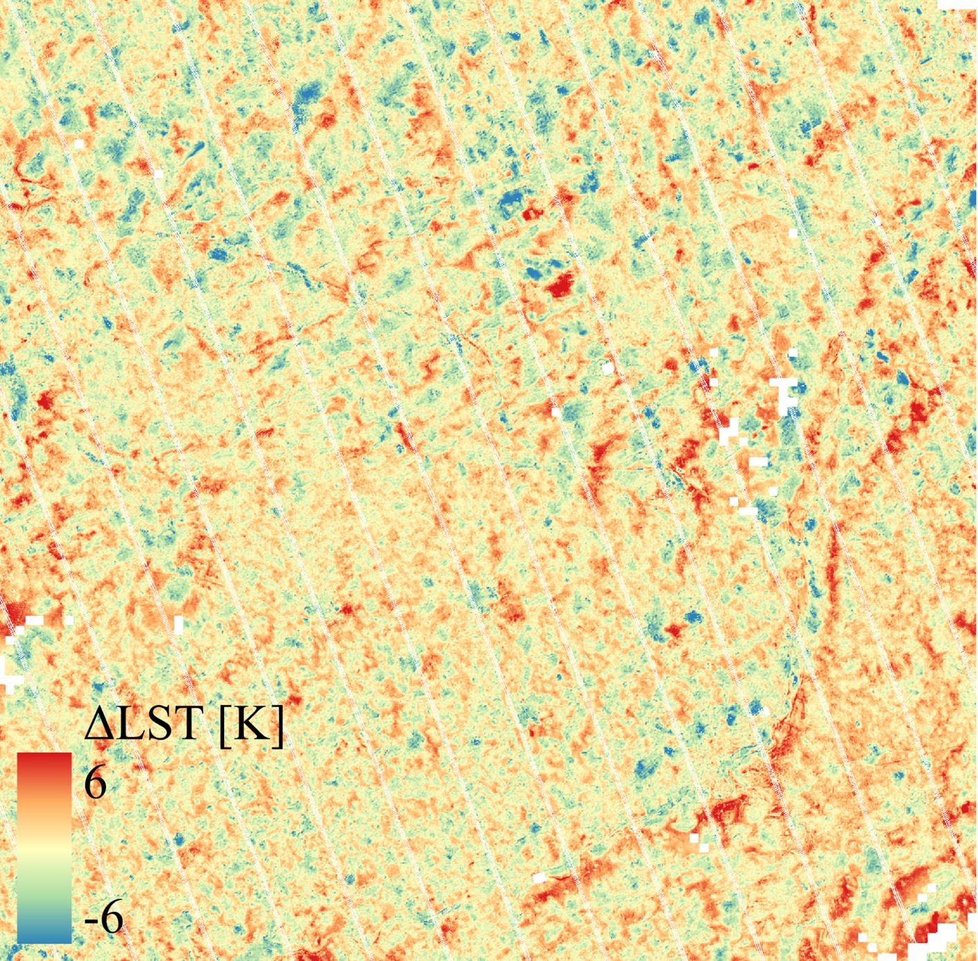
Figure 2: Overview of the sharpening procedure and comparison of the sharpened LST with quasi-simultaneous ECOSTRESS LST for tile 31UFS on 14/06/2022. Fusion of Sentinel-3 (a) and Sentinel-2 (b) resampled to ECOSTRESS (d) provided S3 HR LST (c). Only best quality \pixels, selected by the quality control mask, were used (e) to calculate  between the S3 HR LST and ECOSTRESS LST (f).


Figure 3: Overview of the uncertainties,  , present in the original S3 LST (a), the assumed 2 K uncertainty for the sharpening procedure (b), the uncertainties present in ECOSTRESS LST (c) and the combination of the uncertainties in between the S3 HR LST and ECOSTRESS LST (d) for tile 31UFS on 14/06/2022.

Figure 4: Time series of boxplots representing the ∆LST between S3 HR and ECOSTRESS for the years 2019-2024. The x-axis shows the date of acquisition in DD/MM format.
3.2. Cross-Calibration
Figure 5 presents an overview of S3 HR LST and ECOSTRESS LST for all pixels selected for determining offset and gain for cross-calibration, as described in Section 2.5. The data revealed a clear linear relationship between S3 HR LST and ECOSTRESS LST, spanning from 270 K to 315 K, which was reflected in the cross-calibration line with an R² value of 0.99.
As can be seen in the figure, the data showed an increase in LST spread for increasing temperatures. The trendline, or cross-calibration line, lies above the 1:1 line, indicating higher S3 HR LST values compared to ECOSTRESS LST. This overestimation of S3 HR LST was more pronounced at lower temperatures, despite the smaller spread in LST pairs at these temperatures.
The retrieved gain and offset were used in the next step to cross-calibrate all pixels, including those with different viewing geometries. The dataset, used to derive the gain and offset, where no directional effects were assumed, showed a MAE between S3 HR LST and ECOSTRESS LST of 1.19 K after cross-calibration. This MAE, which is defined as the mean of the absolute difference between the S3 HR LST and ECOSTRESS LST values across all matched pixels, provides an estimate of the inherent uncertainty in the dataset, independent of directional effects.

Figure 5: Density plot of Sentinel-3 HR LST and ECOSTRESS LST for all pixel pairs used in the analysis. The cross-calibration line represents the gain and offset retrieved from the data for calibration of Sentinel-3 data.
3.3. Directional Effects
Gap Effect
The visual identification of the gap effect directly from the pixel pairs was possible by evaluating ΔLST for the difference in viewing zenith angle (VZA), θS3-θECOSTRESS. As a reminder, the gap effect corresponds to observing lower LST for increasing VZA, due to the presence of components with lower temperatures in the line of sight at elevated VZA. If the gap effect was present in the data, ΔLST would decrease for increasing θS3-θECOSTRESS.
Figure 6 illustrates the gap effect. A trendline, representing the ΔLST in a 10° moving window with uncertainty was added to provide a clearer visualization of the overall trend and identification of the underlying gap effect. Within a 10° window, the combination of all pixel pairs determined the average LST difference and average uncertainty:
The uncertainty decreases with the number of independent samples and therefore the uncertainty in the moving window further reduced by the square root of the number of observation pairs, N, within that moving window:
The data revealed a general trend of decreasing temperatures with increasing Δθ, for Δθ ranging from -5° up to 40°. Outside this region, the uncertainty increased due to the reduced number of observation pairs. Additionally, for large Δθ, observation pairs were included for which the S3 LST was influenced by the hotspot. The gap effect was most pronounced for Δθ ranging from 20° to 40°.

Figure 6: Density plot of the ∆LST for ∆θ for all pixel pairs. The moving average shows the trend of the mean ∆LST within the window, including the uncertainty over this value.
The data were further subdivided into four groups based on the time of acquisition and season, resulting in four subgroups: winter morning, summer morning, winter night, and summer night. The subgroups showed slightly different directional effects. Figure 7 illustrates the gap effects of the subgroups. In general, the spread in the data was smaller for colder observations, most notably in the winter night subgroup.
The night observations showed a clear decreasing trend of temperatures as function of increasing ∆VZA. For morning observations, the spread was larger, especially for summer observations. Nonetheless, the general declining trend as function of increasing ∆VZA remained visible. The substantial number of summer morning observations provided additional certainty for the moving average despite the larger spread in the data. The trend in the winter morning observations showed an increase in the 30-45° region. A discussion on the results is given in Section 4.2.
Due to the large spread in the data, the parametric model was used to characterize directional effects of land cover and vegetation density directly. The parametric model provides quantitative results which are easier to interpret. Furthermore, a parametric model allowed to separate and identify gap and hotspot effects. The direct identification of the hotspot effect from the pixel pairs was difficult due to the influence of multiple variables, including zenith angles and relative azimuth angles, θv,S3*HR,i, θv,ECOSTRESS,i, θs, ΔφS3*HR,i and ΔφECOSTRESS,i, which cannot be distinguished in a figure, on the resulting ΔLST.

Figure 7: Density plot of the ∆LST for ∆θ for morning winter, morning summer, night winter and night summer observations. The moving average shows the trend of the mean ∆LST within the window, including the uncertainty over this value
3.4. Directional Models
General model
As described in Section 2.6, the parametric model was fitted to the collection of cross-calibrated pixel pairs, from 2019-2024. Figure 8 presents a polar plot of the directional parametric model for VZA, θv, up to 60°. Modelled directional effects outside the sampling region are not shown, as modelling this region was speculative, because of extrapolation. An observation from the hotspot position resulted in an estimated LST increase of 0.68 K compared to the nadir LST. The modelled directional effects are the largest at high θv opposite to the sun, with LST decreasing up to 1.56 K for θv=50º.
Temporal variations
Since directional effects could have been affected by the time of observation (Duffour et al., 2016b), the dataset was divided into two pairs of subsets: one pair with a winter subset and summer subset and one pair with a morning and night subset. Based on each subset, a separate model was generated as shown in Figure 9 and Figure 10. For the night model, the hotspot kernel was excluded because solar effects did not influence the observed LST. The morning model showed a hotspot peak of 1.10 K and a -1.06 K effect at θv=50º opposite to the Sun. The night model showed a -1.85 K for θv=50º, irrespective of Φv.

Figure 8: Polar plot of the Vinnikov – Roujean-Lagouarde model based on all pixel pairs. The Sun is located at a solar azimuth angle of 150° and a solar zenith angle of 55°.
Furthermore, directional effects may have a seasonal component. Therefore, separate models were fitted for summer and winter observations, as shown in Figure 10. At elevated VZA, the modelled directional effects were more pronounced for the winter model than for the summer model. However, as shown in Figure 7, the winter subset has acquired less pixel pairs for elevated VZA, indicating the modelled directional effects are less reliable at elevated VZA in the winter model. This is confirmed by the instability of the winter model that required an upper boundary of 6 K for the hotspot magnitude B to keep the coefficient values feasible.

Figure 9: Polar plot of the Vinnikov – Roujean-Lagouarde model based on morning and night pixel pairs, respectively. For the morning model, the Sun is located at a solar azimuth angle of 150° and a solar zenith angle of 55°.

Figure 10: Polar plot of the Vinnikov – Roujean-Lagouarde model based on summer and winter pixel pairs, respectively. The Sun is located at a solar azimuth angle of 150° and a solar zenith angle of 45° and 65° for the summer and winter model, respectively.
Land Covers and LAI
The variation in directional effects for various land covers and LAI ranges was reflected in their corresponding models, as shown in Figure 11. The figure shows the variation in the solar principal plane, where the effects are most expressed, for separate land covers (a) and LAI ranges (b).
For water bodies and tree cover, the gap effect was not pronounced, but the hotspot effect was evident, with peaks of 2.48 K and 3.34 K, respectively. Grassland and cropland models showed moderate gap and hotspot effects. In built-up areas, the gap effect was most pronounced, while the hotspot effect was less visible in the figure. However, a significant hotspot effect for built-up was evidenced after comparing the expected LST for θv at opposite sides of the solar principal plane. The model predicted directional effects of -2.83 K for θv=-50º and -0.10 K for θv=50º. The difference of almost 3 K was solely the result of the hotspot effect. Without the hotspot effect, both angles would have shown the same magnitude of directional effects. By evaluating the hotspot effect based on differences in LST along the solar principal plane, tree cover has the largest hotspot effect, followed by built-up, grassland, water and cropland.
The land cover specific models showed an inverse relationship between the hotspot width and the hotspot magnitude. The water bodies and tree cover models showed a narrow peak, whereas the built-up model showed a broad peak, evidenced from the coefficient value and by the presence of positive LST values between the nadir and hotspot position. Since the gap effect is negative, no positive directional effects would have been visible for built-up areas without large hotspot width to counter the effect.
The models derived from pixel pairs assigned to LAI interval indicated a correlation between vegetation density and directional effects. The gap effect was most pronounced for vegetation with low LAI. With increase in LAI values, the magnitude of the gap effect decreased, eventually converging towards zero for LAI values above 2. The models showed an opposite trend for the magnitude of the hotspot effect. A small hotspot effect was characterized by the model for vegetation with low LAI, while the hotspot magnitude was highest for the vegetation in the highest LAI interval, peaking at 3.34 K. Additionally, the hotspot width increased as the magnitude decreased, although this trend was less pronounced compared to the different land covers.


Figure 11: Modelled directional effects by the Vinnikov – Roujean-Lagouarde model in the solar principal plane for a range of land covers and leaf area index (LAI) intervals. The Sun is located at a zenith angle θs of 55°. The land cover models are based on pure pixels. The LAI models are based on pixels with an LAI value and corresponding to a natural land cover.
Summarizing Tables
Table 2 and Table 3 provide an overview of the model coefficients retrieved for each dataset and a corresponding comprehensive overview of the modelled directional effects in the solar principal plane, respectively. The tables include models for general observations, temporal variations, seasonal variations, land covers, and LAI intervals. Table 2 also includes confidence intervals (CI) for each coefficient, estimated by bootstrapping the datasets, as explained in Appendix C. Note, the values of modelled effects are extracted for a specific θs that was set to 45° for the summer model, 55° for models including observations throughout the year and 65° for the winter model. Furthermore, no Sun was present for the night model. All expected LST changes attributed to directional effects were within reasonable bounds, as these effects are the result of component temperature differences in the observed scene, which can vary by some Kelvins. However, the modelled LST changes for the winter model might be unreliable due to instability in parameter retrieval. For the same reason, no 95% CI could be established for hotspot coefficient B.
The uncertainties in gap coefficient A and the hotspot magnitude coefficient B were approximately normally distributed, as reflected in their 95% CIs. In contrast, the uncertainty was not normally distributed for the hotspot width k due to the exponential nature of the hotspot kernel, see equation (12). This resulted in CIs that spanned several orders of magnitude.
Figure 12 shows the sensitivity of the general model to changes in hotspot width. The figure clearly shows that for very small k values, below 10-6, the model is almost insensitive to changes in k, which explains the wide range in some of the 95% CIs.
Table 2: Summary of parameter coefficients for various models, including the 95% Confidence Interval (CI).
| A [K] | 95% CI [K] | B [K] | 95% CI [K] | k [-] | 95% CI [-] | |
|---|---|---|---|---|---|---|
| General | -1.34 | [-1.58, -1.13] | 1.26 | [1.13, 1.37] | 2.97·10-9 | [1.14·10-9, 4.94·10-5] |
| Morning | -0.19 | [-0.40, -0.00] | 1.16 | [1.06, 1.26] | 8.84·10-8 | [3.42·10-9, 1.15·10-5] |
| Night | -5.15 | [-5.32, -4.98] | N/A | N/A | N/A | N/A |
| Winter | -5.19 | [-5.32, -5.06] | 6.00 | N/A | 4.12·10-8 | [8.85·10-9, 3.76·10-7] |
| Summer | -1.13 | [-1.37, -0.90] | 1.16 | [1.05, 1.28] | 1.14·10-5 | [5.76·10-9, 1.62·10-2] |
| Land cover | ||||||
| Water | ≈ 0 | [-7.78·10-6, -8.44·10-9] | 2.80 | [2.26, 3.36] | 2.94 | [2.65, 3.21] |
| Tree cover | ≈ 0 | [-1.14·10-8, 0] | 3.37 | [2.79, 3.98] | 2.04 | [1.65, 2.45] |
| Cropland | -2.07 | [-2.29, -1.83] | 1.14 | [1.01, 1.29] | 7.08·10-6 | [1.43·10-9, 0.13] |
| Grassland | -0.73 | [-0.95, -0.50] | 1.41 | [1.29, 1.52] | 9.19·10-7 | [6.39·10-9, 5.40·10-5] |
| Built-up | -4.01 | [-4.31, -3.71] | 1.61 | [1.46, 1.75] | 1.36·10-7 | [6.29·10-9, 1.68·10-5] |
| LAI | ||||||
| [0, 0.25] | -6.25 | [-6.54, -5.96] | 0.78 | [0.64, 0.92] | 7.79·10-7 | [8.00·10-9, 2.38·10-5] |
| [0.25, 0.50] | -3.83 | [-4.18, -3.41] | 2.75 | [1.48, 3.94] | 1.76 | [0.57, 2.44] |
| [0.50, 0.75] | -1.80 | [-2.08, -1.51] | 2.62 | [1.44, 3.71] | 2.03 | [0.89, 2.71] |
| [0.75, 1] | -1.25 | [-1.51, -1.01] | 3.39 | [2.39, 4.55] | 2.49 | [1.78, 3.06] |
| [1, 2] | -0.35 | [-0.60, -0.12] | 2.40 | [1.66, 3.22] | 1.56 | [0.81, 2.22] |
| [2, 8] | ≈ 0 | [-6.67·10-8, 0] | 3.35 | [2.78, 3.96] | 2.31 | [1.93, 2.66] |
Table 3: Summary of expected LST at different viewing zenith angles relative to nadir LST in the solar principal plane for various conditions, including the expected LST directional effect at the hotspot position with solar zenith angle.
| -50° [K] |
-35° [K] |
-20° [K] |
20° [K] |
35° [K] |
50° [K] |
θs [°] | Hotspot [K] | |
|---|---|---|---|---|---|---|---|---|
| General | -1.56 | -0.87 | -0.41 | 0.24 | 0.37 | 0.56 | 55 | 0.68 |
| Morning | -1.06 | -0.62 | -0.31 | 0.29 | 0.54 | 0.91 | 55 | 1.10 |
| Night | -1.85 | -0.94 | -0.31 | -0.31 | -0.94 | -1.85 | — | — |
| Winter | -5.19 | -2.90 | -1.33 | 0.71 | 1.02 | 1.48 | 65 | 3.01 |
| Summer | -1.82 | -1.04 | -0.50 | 0.36 | 0.61 | 0.53 | 45 | 0.83 |
| Water | -0.04 | -0.04 | -0.03 | 0.08 | 0.27 | 1.23 | 55 | 2.48 |
| Tree cover | -0.18 | -0.15 | -0.10 | 0.20 | 0.27 | 1.20 | 55 | 3.84 |
| Cropland | -1.73 | -0.95 | -0.42 | 0.17 | 0.18 | 0.21 | 55 | 0.25 |
| Grassland | -1.46 | -0.84 | -0.40 | 0.18 | 0.16 | 0.03 | 55 | 0.28 |
| Built-up | -2.83 | -1.54 | -0.66 | 0.17 | 0.07 | -0.09 | 55 | -0.10 |
| LAI | ||||||||
| [0, 0.25] | -2.92 | -1.54 | -0.59 | -0.16 | -0.72 | -1.54 | 55 | -1.83 |
| [0.25, 0.50] | -1.59 | -0.87 | -0.35 | -0.02 | -0.11 | 0.11 | 55 | 1.24 |
| [0.50, 0.75] | -0.81 | -0.45 | -0.19 | 0.07 | 0.15 | 0.45 | 55 | 1.81 |
| [0.75, 1] | -0.56 | -0.32 | -0.14 | 0.07 | 0.25 | 1.41 | 55 | 2.89 |
| [1, 2] | -0.39 | -0.26 | -0.15 | 0.20 | 0.51 | 1.87 | 55 | 3.31 |
| [2, 8] | -0.12 | -0.11 | -0.07 | 0.17 | 0.52 | 1.89 | 55 | 3.34 |

Figure 12: Modelled directional effects by the Vinnikov – Roujean-Lagouarde model in the solar principal plane for varying hotspot widths k. The Sun is located at a zenith angle θs of 55°.
3.5. Validation of Correction Strategy
3.5.1. General Correction
Figure 13 illustrates the distribution of ΔLST for all acquisition pairs in the validation year 2023, comparing the original data, cross-calibrated data, and directionally corrected data. The overall performance was evaluated by combining all pixel pairs into a single dataset. Both cross-calibration and directional correction reduced the absolute value of the median ΔLST. Additionally, the directional correction decreased the spread in the dataset compared to the cross-calibrated dataset.
Overall, the mean ΔLST, to which we refer as the mean error (ME), decreased from the original ME of 1.22 K to -0.25 K after cross-calibration and to -0.22 K after directional correction. This metric indicated a shift from an overestimation of S3 HR compared to ECOSTRESS to an underestimation after directional correction, which was still present but reduced.
The mean absolute error (MAE), which quantifies the average magnitude of LST differences regardless of direction, improved from 1.68 K to 1.61 K after cross-calibration and further to 1.48 K after directional correction. Although the largest shift in ΔLST was observed after cross-calibration, it has only a minor influence on the MAE compared to the directional correction. Assuming the MAE of 1.19 K for pixel pairs without directional differences, as described in Section 3.2, represents the baseline uncertainty, 31% of directional effects were removed by the general model:

Figure 13: Time series of boxplots showing the ΔLST between S3 HR and ECOSTRESS for the validation year 2023. The x-axis displays the acquisition dates in DD/MM, with results shown for the original, cross-calibrated, and directionally corrected data.
3.5.2. Case-Specific Corrections
The time-of-day correction utilized two models: a morning model and a night model. The validation data was corrected according to the model corresponding to each acquisition pair. Additionally, combining different strategies enabled further differentiation of models. However, in some cases this led to numerous directional models required for the correction strategy, as was the case for the land cover + time of day (tod) correction with ten models, one for each of the five land covers for morning and for evening observations. Table 4 provides an overview of all tested correction strategies, each showing improvements in both ME and MAE.
Each correction strategy outperformed the general correction strategy, with the time-of-day strategy demonstrating the largest MAE decrease, up to 1.33 K. This corresponds to a 66.7% removal of directional effects, taking the MAE of 1.19 K, as described in Section 3.2, as baseline:
A correction strategy for different LAI ranges was also evaluated but not included in the table, as it required a different original dataset with only pixels having LAI values. For the correction based on LAI interval specific models, the original LAI dataset had ME values of 1.23 K, -0.05 K, and 0.01 K for the original, cross-calibrated, and directionally corrected datasets, respectively. The MAE improved from 1.70 K to 1.59 K to 1.45 K.
Table 4: Comparative performance assessment of different correction strategies based on Mean Error (ME) and Mean Absolute Error (MAE) of the directionally corrected data.
| ME [K] | MAE [K] | |
| General | -0.22 | 1.48 |
| Time of day (tod) | -0.12 | 1.33 |
| Season | -0.16 | 1.45 |
| Tod + season | -0.13 | 1.38 |
| Land cover | -0.20 | 1.47 |
| Land cover + tod | -0.10 | 1.34 |
| Land cover + season | -0.15 | 1.44 |
| Land cover + tod + season | -0.10 | 1.38 |
4. Discussion
4.1. Observation Pairs Comparison and Cross-Calibration
The 10-minute interval between S3 and ECOSTRESS acquisitions resulted in 60 observation pairs. This time interval was not chosen arbitrarily but follows the guidelines of the Land Surface Temperature Product Validation Best Practice Protocol (Guillevic et al., 2018). Temperature changes can still occur within this time interval, especially for morning observations, when the temperature gradients are high. To estimate the temporal effect, we combined the Diurnal Temperature Cycle (DTC) proposed by Göttsche & Olesen (2001) with a diurnal temperature range of 15 K and a peak temperature time at 13:00, representative values for Flanders in July (Sharifnezhadazizi et al., 2019). By setting the DTC width to 14 hours, in line with Göttsche & Olesen (2001), a temperature gradient at 10:00 of approximately 2.1 K/h was estimated. This implies an average temperature change of 0.35 K within the 10-minute interval for morning observations in July. This marks an upper limit estimate, as temperature gradients are typically smaller during other months and for night observations. Since ECOSTRESS acquisitions occur both before and after the S3 acquisitions, and linear effects can be assumed over the small time interval, the temporal effects tend to cancel out, which minimizes impact on coefficient fitting.
Extension of the time interval to 20 minutes would approximately double the number of observation pairs. However, it also increases uncertainty in the comparison of the two datasets due to more pronounced temporal gradients. An assessment of the trade-off lies beyond the scope of this study. Nevertheless, for future satellite missions LSTM, TRISHNA and SBG, extending this time interval for selecting observation pairs might be beneficial. These missions acquire data around noon, when temperature gradients are minimal.
Figure 3 shows that both the native LST errors from S3 and ECOSTRESS, as well as the sharpening process contribute to reduced accuracy in the ΔLST of the pixel pairs. The sharpening process, with an estimated uncertainty of 2 K, is the dominant source of the final uncertainties, which are only slightly higher than the defined sharpening uncertainty. This illustrates the disadvantage of using the sharpening procedure to obtain HR LST. There is a significant opportunity for future native HR thermal datasets to replace the sharpened data in the presented methodology to fit directional coefficients. Nonetheless, the effect of the large uncertainty present in the data is countered by using a large dataset.
The overestimation of S3 LST compared to ECOSTRESS LST is visible in most individual observation pairs and in the overall cross-calibration data, as shown in Figure 4 and Figure 5, respectively. This overall bias is the result of the hot bias in S3 (Pérez-Planells et al., 2021; Sanchez et al., 2024) and the cold bias in ECOSTRESS, which is more expressed for lower LST values, below 295 K, due to an issue during the post-launch calibration (Hu et al., 2022; Hulley et al., 2021). As a result, S3 LST overestimation, relative to ECOSTRESS LST, is most pronounced at the lower LST range. These biases reinforce the rationale for the cross-calibration.
Despite the decrease in LST accuracy for thermally sharpened products (Gao et al., 2012), the comparison of S3 HR LST with ECOSTRESS, under similar viewing conditions, reveals a strong correlation, reflected by an R² value of 0.99 in Figure 4. This justifies the use of ECOSTRESS for evaluating directional effects in the thermally sharpened S3 data. However, the LST uncertainty, reflected by the ΔLST spread, increases for higher LST. This effect is the result of the loss in thermal contrast in sharpened images, which affects observations at the higher end of the LST range in the dataset the most (Guzinski & Nieto, 2019; Sanchez et al., 2024). Guzinski et al. (2023) offers a solution by comparing the coefficient of variation of sharpened S3 LST with Landsat LST to increase the thermal contrast. While we did not apply this method, the increased uncertainty introduced by the sharpening procedure is countered by the large data pool, 60 observation pairs, in our study, which shows to be sufficient to estimate the gain and offset between the datasets and thus mitigate the impact of the reduced LST accuracy on the results.
Due to the strong correlation between the two datasets, after screening for acquisition geometry, the cross-calibration removes the main LST differences. The remaining differences can be assumed to be random noise and directional effects.
4.2. Directional Effects
The general trend of decreasing temperatures with increasing differences of viewing zenith angles, Δθ, in the density plots suggests that the viewing zenith angle significantly influences the recorded LST and thus confirms the gap effect, which was previously identified in literature (Bian et al., 2025; Michel et al., 2023; Vinnikov et al., 2012). Furthermore, for small Δθ, where no directional effects are expected, the moving average of ΔLST is close to 0 K, as shown in Figure 6, which also confirms the successful cross-calibration. The ΔLST spread in this region shows the large uncertainty in the data non-related to directional effects, including S3 LST uncertainty, sharpening uncertainty and ECOSTRESS LST uncertainty.
The gap effect is most visible in the density plots of the night subgroups since it is the only directional effect present, due to the absence of the Sun. Vinnikov et al. (2012) exploits this characteristic by retrieving the gap coefficient solely from night observations to isolate gap effects without the influence of solar radiation. Furthermore, the colder night observations, especially during the winter, contain less thermal contrast, which improves the accuracy of S3 HR estimates and thus reinforces the observed gap effect for these observations, due to the smaller spread in ΔLST. The larger spread for morning observations, particularly in summer, highlights the vulnerability of thermal sharpening of acquisitions containing large thermal contrast (Guzinski & Nieto, 2019).
The visualisation of the hotspot effects directly from the data is difficult due to the larger number of influencing variables, as mentioned in Section 3.2. Furthermore, the identification of the hotspot effect is less straightforward for two reasons. Firstly, the gap effect is strictly negative (B. Cao et al., 2019) and thus induces a counteractive directional effect for the strictly positive hotspot effect, resulting in dome and bell-shaped signature patterns (B. Cao et al., 2021). The fact that the solar zenith angles (SZAs) in Flanders are large at 10:00 coordinated universal time (UTC), ranging from 34° and 77°, means that when the satellite is positioned in the neighbourhood of the solar direction, the satellite viewing zenith angle (VZA) is large and thus the gap effect plays a significant role. Secondly, observations close to the hotspot peak, i.e. within 13° and 7° for ECOSTRESS and S3, respectively, where the exponential hotspot effect is most expressed, are not present. The absence of observations for small phase angles, where the viewing angles and solar angles are similar, despite 60 observation pairs, reveals the difficulty to get an impression of the hotspot peak for the region of Flanders, which is the case for all regions at higher latitudes.
4.3. Directional Models
General Model
The general model in this study is in accordance with parametric models earlier derived from the combination of twelve Master airborne tracks in Southern California (Michel et al., 2023). The models from that airborne campaign estimate directional effects in the same order of magnitude. Among the models tested by Michel et al. (2023), the LSF-RL model has a shape most closely resembling the Vinnikov-RL shape. The parameters of their LSF-RL model are: k1=-0.047 LSTnadir, k2=0.0058 LSTnadir, khs=9.7 10-7. Assuming an average LSTnadir of 290 K, k1 and k2 become -13.6 K and 1.68 K, respectively. Figure 14 provides a direct comparison of the directional effects modelled by our general Vinnikov-RL and their LSF-RL model in the solar principal plane, where directional effects are most pronounced. Despite differences in gap kernel definition, methodology, data and region, the figure reveals a strong similarity between the two models. Our estimated hotspot magnitude B=1.26 K is slightly lower than their 1.68 K. However, our hotspot width coefficient k=2.97 10-9 is much higher than their 9.7 10-7. Nevertheless, as illustrated in the figure, for very low values, modelled effects are little affected due to the characteristics of the RL kernel.

Figure 14: Comparison of our general Vinnikov-RL model and the global LSF-RL model derived by Michel et al. (2023) for a nadir temperature of 290K in the solar principal plane for a solar zenith angle of 55°.
The general Vinnikov-RL directional model indicates that directional effects influence LST up to approximately 1.6 K, as shown in Table 3. Even for θv =35º, the maximal VZA for the upcoming thermal IR missions LSTM (Koetz et al., 2021), TRISHNA (Charvet et al., 2022) and SBG, the observed temperatures are affected up to 0.9 K. The modelled directional effects in this study endanger the user requirements specified accuracy of 1 K needed for precision agriculture applications, including water stress detection and evapotranspiration estimation (Sobrino et al., 2016), which are primary objectives of LSTM and TRISHNA. Combined with other uncertainties, inherently present in TIR dataset, the specified accuracy will not be met. Therefore, a directional correction is advised.
Furthermore, the average SZA of 55° in our study corresponds to elevated latitudes in Flanders around 51° at 10:00. However, the SZA is a variable. Future LSTM, TRISHNA and SBG observations will face lower SZA during summer season or when observing regions located at lower absolute latitudes. Additionally, these missions aim for a local solar time in the early afternoon, since thermal contrast and crop water stress is maximal when the SZA is minimal (Koetz et al., 2021; Udelhoven et al., 2017). For smaller directional effects will further degrade LST measurements due to the larger influence of the hotspot closer to the nadir direction. These results underscore the necessity of accounting for directional effects using appropriate directional models.
Time-specific Models
This study considers separate morning and night models and winter and summer models, since directional effects are time dependent (Na et al., 2024; Qin et al., 2023). One simulation study (Duffour et al., 2016b) found that directional effects are more expressed during day and summer period. The direct comparison between modelled directional effects for morning and night observations is difficult due to the differences in solar conditions. Nonetheless, opposite to the sun, the directional effects are slightly more expressed in morning observations, as shown in Table 3. A potential explanation is the larger temperature difference between scene components during the day, which drives the gap effect.
The comparison of the winter and summer model shows the opposite behaviour. The modelled directional effects are stronger in the winter model, despite the generally larger temperature differences between scene components during the summer. However, the fitting of the resulting winter model resulted in the hotspot coefficient reaching the upper boundary, which indicates an unstable optimization. This might be the result of insufficient sampling in the hotspot region.
For winter observations, observed pixels closest to the solar position still more than 30° away from this position, which means that even the closest pixels lie in the tail of the modelled exponential hotspot. This makes the peak magnitude, represented by the hotspot coefficient, estimation sensitive to the data. There are only four out of a total of ten winter morning observation pairs, with VZAs above 30°. Therefore, these four observation pairs almost solely influence the hotspot estimation. Furthermore, one of these four observation pair, on 16/10/2022, is responsible for the most dense region in the winter morning density plot, corresponding to the sudden ∆LST increase, shown in Figure 7. The combination of the sensitivity of the hotspot estimation and the high ∆LST for the largest observation pair, which is also among the observations closest to the solar position results in an hotspot peak overestimation, and therefore hotspot coefficient converged to the upper boundary.
The extrapolation problem is more expressed in winter for two reasons. First, the θs is larger in winter than in summer and second, in the dataset, the maximum θv values were lower for winter observations than for summer observations. As a result, in the winter model the incorrectly modelled hotspot effect also increases the modelled gap effect to compensate for the elevated temperatures, which gives an underestimation of modelled temperatures opposite to the solar position. The results indicate the difficulty of estimating the hotspot kernel in case of insufficient sampling close to the solar position. Therefore, we do not recommend building a separate winter model in case observations provide poor sampling, which is the case for regions located at higher latitudes.
Land cover and LAI Models
Figure 11 shows that models constructed for the most heterogenous scenes, such as built-up, show the largest gap effects, contrary to the homogenous land covers: water and tree cover. For land covers that have mixed homogenous and heterogenous structure, such as grassland and cropland, the gap effect is intermediate. The trend in gap effects is also confirmed by the constructed models for different LAI ranges, representing differences in canopy density. For vegetation with low LAI, which is more heterogeneous, gap effects will be large, whereas for homogeneous vegetation, i.e. LAI values above 2, there is no gap effect.
An explanation for the observed phenomenon is the more complex scene 3D structure that changes the observed LST significantly for varying viewing geometry. This is not the case for water or dense forests, where regardless of the viewing angle, water and forest canopy is observed. Within the cropland and grassland class, there is a larger distribution of dense and sparse scenes. For fully grown crop fields, with high LAI values, the gap effect will be smaller, since it is more homogenous than for early growth crop fields, with small LAI values, where the gap effect will be more significant since the scene is more heterogeneous. The combination of all cropland and grassland will therefore be a mixture of directional effects and gives intermediate results.
There is a large similarity between the tree cover model and the model for the [2:8] LAI range, which is obvious due to the overlap in dataset characteristics. Both models show no gap effect but do show large hotspot effects. This is possibly the result of the multilayer canopy that blocks soil radiation but still introduces shadowing effects in the canopy itself. The results are in line with directional effects observed in a laboratory setup, which showed that dense forests are more prone to the hotspot effect due to the presence of sunlit leaves and sparse forests are more prone to the gap effect (Adams et al., 2025).
Prior anisotropy measurements from (Duffour, Lagouarde, & Roujean, 2016) from multi-angular airborne campaigns over Toulouse (Lagouarde & Irvine, 2008) and over a forest canopy (Lagouarde et al., 2000) confirm the modelled dominant gap effect over urban areas and the minor gap effect for a forest canopy. Furthermore, the airborne measurements confirm that the hotspot effect is wide for urban areas and narrow for forests.
Our study’s findings confirm the presence of both gap and hotspot effects in thermally sharpened images, which were earlier observed for a limited range of landscapes in HR surface brightness temperatures (Michel et al., 2023). Michel et al. (2023) concluded that directional effects in urban areas and in low vegetation with low NDVI are comparable, aligning with our results where built-up areas exhibit strong gap effects due to structural heterogeneity. Furthermore, they found that directional effects vary with NDVI levels, an observation that matches our LAI models, where canopy density determines the magnitude of gap and hotspot effects. However, the authors noted that the combination of limited data and mixed pixels at a 100 m resolution resulted in average directional trends, preventing reliable land cover modelling. In contrast, our land cover analysis benefits from a larger dataset composed solely of pure pixels, enabling a clearer separation of directional effects and modelling for the identified land covers.
The results nuance the findings of (Duffour et al., 2016b), which uses a single number, the directional anisotropy index (DAI). In contrast, our study separates gap and hotspot effects, revealing that these effects behave differently to changes in canopy structure and land cover, thus providing detailed understanding of directional effects behaviour. Furthermore, the resulting trends in the constructed directional models are in line with the trends in directional models for heterogenous and homogenous landscapes based on low spatial resolution MODIS observations (Hu et al., 2023).
4.4. Correction Strategies
Previous studies proposed global correction strategies for low-resolution LST (Na et al., 2024; Vinnikov et al., 2012), or local correction strategies for HR LST (Michel et al., 2023). However, the novel framework in this study provides a first directional correction strategy for HR LST that can be applied on a global scale if S3, S2 and ECOSTRESS observations are available, paving the way for a first operational correction.
All correction strategies show a decrease in ME and MAE between the two LST datasets. The results show that the cross-calibration step is most effective for bias corrections, reflected by the ME, whereas the directional correction improves the accuracy, reflected by the MAE, of the observed LST.
Although the results from the correction based on the general model indicate a reduction in bias and an enhancement in accuracy, the MAE decreases more for case-specific approaches. The results from the different correction strategies indicate that evolving towards case specific corrections, especially for time-of-day, is advised. Separating morning and night models significantly outperforms the general correction strategy, which suggests that estimating the gap effect from night observation to correct for gap effects in morning acquisitions might not be a good practice and should only be considered when no other options are available (Vinnikov et al., 2012). Combining different correction strategies does not further enhance accuracy. This suggests that integrating multiple factors that influence LST measurements can lead to less robust correction models. The number of acquisition pairs and the sampling within these subdatasets have an influence on the construction of models.
Considering the MAE of 1.19 K for the pixel pairs used for cross-calibration, i.e. where no directional effects are assumed, as baseline, 31% and 67% of the directional effects are removed by the general correction strategy and the tod correction strategy, respectively.
The resulting MAE decreasing from 1.61 K, after cross-calibration, to 1.48 and 1.33 K, after directional correction, is a modest improvement. The inherent uncertainties in the S3 and ECOSTRESS data, in nadir and oblique observations, combined with uncertainty introduced by the sharpening algorithm, as described in Section 2.3, prohibit reaching larger improvements.
Nevertheless, the proposed methodology succeeds modelling and reducing a portion of directional effects, demonstrating that these corrections are feasible even with suboptimal data. Future HR LST datasets are expected to have significantly lower intrinsic uncertainty. The amplitude of the directional effects is such that the corrections will be needed to reach the desired 1 K threshold for precision agriculture (Sobrino et al., 2016), required to allow ET estimates to be within 10% relative error (Fisher et al., 2017).
4.5. Operational Context
4.5.1. Applicability to Other Regions
Flanders, located at a latitude of 51°N, provides a diverse landscape including cropland, grassland, urban areas, forests and water bodies, making it a representative case for comparable regions in Europe. The derived directional model coefficients are expected to be applicable to neighbouring regions such as the Netherlands, northern France and western Germany. These regions share comparable topography, vegetation structure, and land cover composition, which supports the extension of the model. Other regions may benefit from recalibrating the directional coefficients, an exercise that falls outside the scope of this paper.
It is important to distinguish between the general model and the case-specific corrections. The general model, trained on a large and diverse dataset, provides a robust baseline correction that can be applied operationally with limited ancillary data. Contrary, case-specific models, such as the land cover models, offer a more differentiated correction but require additional input data. These models also benefit from recalibration when applied to new regions, especially in case of different climate types. Although the study is limited to Flanders, the developed methodology is designed to be transferable to other geographic areas. This flexibility allows the methodology to adapt to a wide range of geographic and climatic contexts, except for regions above 52° latitude where no ECOSTRESS acquisitions are available.
4.5.2. Relevance for Upcoming High-Resolution Thermal Missions
The proposed methodology is particularly relevant in the context of upcoming high-resolution thermal missions such as LSTM, TRISHNA, and SBG. These missions are designed to deliver native HR LST products with targeted accuracies below 1 K. Key distinctions between the context of our study and the context of these missions are the maximum VZA, time of acquisition and corresponding SZA, radiometric accuracy and revisit frequency.
S3 LST is acquired with acquisition angles above 50°, in contrast to the upcoming high-resolution thermal missions, that aim for a maximum VZA of 34° in case of SBG and TRISHNA, and 28° in case of LSTM. However, when deriving directional coefficients from these missions, their application to data retrieved from the same satellite is valid, since both sampling and correction occur within the same VZA range.
The SZA varies with latitude, time of day and time of year. This study focuses on observations around 10:00 local time. In contrast, TRISHNA, SBG and LSTM are designed to acquire data around 12:30-13:00 local time, when SZA is lowest and thermal contrast is highest (Koetz et al., 2021). As a result, for these missions the hotspot influence will be more expressed at lower zenith angles, especially for regions at lower latitudes. However, the retrieval of hotspot coefficients also improves when the effect is more pronounced at lower zenith angles.
The methodology would benefit from replacing S3 with native high-resolution thermal data from LSTM, TRISHNA and SBG as it increases radiometric accuracy of the data for which the directional coefficients are retrieved, especially for case-specific coefficients. Individually these missions deliver less frequent acquisitions, resulting in less observation pairs. However, the methodology would benefit from the synergy of the three datasets, leading to combined daily revisits.
Important to note is that the irregular orbit of ECOSTRESS enables the construction of a dataset with quasi-simultaneous acquisitions. In case ECOSTRESS data is no longer available, an alternative dataset needs to be incorporated. With recent developments in thermal remote sensing and corresponding future increased thermal capabilities, several datasets might serve as potential replacement of ECOSTRESS in the proposed methodology.
If the final designs of LSTM, TRISHNA and SBG allow for occasional simultaneous acquisitions, this would allow to cross-calibrate data and model directional effects. Our methodology could exploit this feature, resulting in three sets of observation pairs: LSTM-TRISHNA, THRISNA-SBG and SBG-LSTM. Furthermore, emerging commercial space companies, such as Ororatech and Constellr, may offer additional comparative data through their thermal satellite constellations, further increasing the possible data usable in our proposed methodology.
In conclusion, the developed methodology not only addresses current limitations in HR LST retrievals but also provides a potential solution for correcting future thermal datasets. Correcting for directional anisotropy supports the delivery of reliable LST products that meet the stringent requirements of future satellite missions.Click or tap here to enter text.
4.6. Limitations
The main limitation of this study is the use of data that contain high uncertainty, inherently present in the LST values. As a result, the relative impact of directional effects on the data is limited, and thus so is any directional correction. This large uncertainty, mainly introduced by the sharpening procedure, complicates the validation exercise. However, due to the large number of observation pairs, we still get feasible results and even be able to differentiate models for the time of day, land cover and LAI. Only the construction of a feasible model for the winter observations is difficult due to the lack of sampling close to the solar position, leading to mismodelling the hotspot effect, especially the peak.
5. Conclusion
This study presents a novel approach to identify and correct directional effects in high-resolution (HR) LST, synthetically generated using the Data Mining Sharpener (DMS). To overcome the lack of HR LST datasets suitable for researching directional effects, we generated sharpened Sentinel-3 (S3) LST for simultaneously acquired ECOSTRESS LST. A cross-calibration based on LST acquired under similar viewing conditions revealed an overestimation in S3 LST compared to ECOSTRESS. After calibration, a baseline Mean Absolute Error (MAE) of 1.19 K was achieved, representing the inherent uncertainty unaffected by directional effects.
The collection of thermal observation pairs with view zenith angles (VZA) up to 50°, enabled the identification and characterization of directional effects in HR LST. This marks the first framework capable of assessing directional effects in HR thermal data at a global scale. Our findings confirm the presence of both gap and hotspot effects.
Furthermore, despite the large uncertainties associated with the data, we were capable constructing a parametric model. Combining a Vinnikov gap kernel and a Roujean-Lagouarde hotspot kernel allowed quantifying the magnitude of these gap and hotspot effects. The general model, based on the whole dataset, simulates directional effects in the solar principal plane ranging from -0.87 K to 0.37 K for a VZA up to 35°, and from -1.56 K to 0.56 K for a VZA up to 50°. These results highlight the importance of considering directional effects in both thermally sharpened and native HR LST.
The gap effect is most pronounced in heterogeneous surfaces, such as built-up areas, with -2.8 K, and low LAI vegetation, with -2.9 K, at 50º VZA. Contrary, the hotspot effect is dominant in homogenous vegetation, particularly for tree cover, with a peak temperature of 3.3 K.
Although the correction strategies showed a moderate reduction in MAE between S3 and ECOSTRESS LST, due to the high inherent uncertainties, substantial reductions in directional effects were accomplished. The time-of-day specific models, separating morning and night observations, yielded the most promising results with a 67% decrease in directional effects. The results demonstrate the potential of case-specific corrections and emphasize the importance of building separate daytime and nighttime models in operational algorithms.
The analysis in this study is limited to Flanders, located at a latitude of 51°N. However, given the diversity of land cover types across this area, we expect the findings to be broadly applicable to other regions with a temperate climate.
This study establishes a solid foundation for advancing directional correction methods in future high-resolution LST applications. With upcoming satellite missions such as LSTM, TRISHNA and SBG that will deliver native HR LST with targeted accuracies below 1 K, necessary for precision agriculture applications, the impact of directional effects will become more pronounced and should be addressed. Furthermore, these new datasets will enable more refined analyses, including pixel-specific corrections considering a variety of land covers and associated dynamic conditions.
Concluding, this research provides a novel and almost globally applicable methodology for detecting and correcting directional effects in HR LST. This is an important step towards an operational correction strategy that meets the stringent accuracy requirements of precision agriculture and other Earth Observation applications.
Author Contributions
Louis Snyders: Conceptualization, Methodology, Software, Validation, Formal analysis, Investigation, Data Curation, Writing – Original Draft, Funding acquisition. Joris Blommaert and Jonathan León-Tavares: Writing – Review & Editing, Supervision, Funding acquisition, Project administration. Jeroen Degerickx: Methodology, Software, Resources, Writing – Review & Editing, Supervision, Funding acquisition, Project administration
Declaration of Competing Interests
The authors declare that they have no known competing financial interests or personal relationships that could have appeared to influence the work reported in this paper.
Acknowledgements
The authors thank the associate editor and the reviewers for their systematic review and valuable comments.
Funding
This work is the result of (1) being selected via the Open Space Innovation Platform (https://ideas.esa.int) as a Co-Sponsored Research Agreement and carried out under the Discovery programme of, and funded by, the European Space Agency, which was awarded to Louis Snyders, and (2) the ESA EO AfRIca ExplorerS project (ARIES – contract nr. 4000139191/22/I-DT), managed by Jeroen Degerickx for VITO.
References
Adams, J. S., Damm, A., Werfeli, M., Gröbner, J., & Naegeli, K. (2025). Across-scale thermal infrared anisotropy in forests: Insights from a multi-angular laboratory-based approach. Remote Sensing of Environment, 326, 114766. https://doi.org/10.1016/J.RSE.2025.114766
Agam, N., Kustas, W. P., Anderson, M. C., Li, F., & Neale, C. M. U. (2007). A vegetation index based technique for spatial sharpening of thermal imagery. Remote Sensing of Environment, 107(4), 545–558. https://doi.org/10.1016/J.RSE.2006.10.006
Ambas, V. T., & Baltas, E. (2012). Sensitivity analysis of different evapotranspiration methods using a new sensitivity coefficient. Global NEST Journal, 14(3), 335–343.
Bian, Z., Roujean, J. L., Irvine, M., Li, H., Mo, F., Chen, Y., Cao, B., Du, Y., Xiao, Q., & Liu, Q. (2025). Evaluation of three modelling frameworks of thermal infrared radiative transfer for directional anisotropies of temperatures. IEEE Transactions on Geoscience and Remote Sensing. https://doi.org/10.1109/TGRS.2025.3530503
Cao, B., Gastellu-Etchegorry, J. P., Du, Y., Li, H., Bian, Z., Hu, T., Fan, W., Xiao, Q., & Liu, Q. (2019). Evaluation of Four Kernel-Driven Models in the Thermal Infrared Band. IEEE Transactions on Geoscience and Remote Sensing, 57(8), 5456–5475. https://doi.org/10.1109/TGRS.2019.2899600
Cao, B., Roujean, J.-L., Gastellu-Etchegorry, J.-P., Liu, Q., Du, Y., Lagouarde, J.-P., Huang, H., Li, H., Bian, Z., Hu, T., Qin, B., Ran, X., & Xiao, Q. (2021). A general framework of kernel-driven modeling in the thermal infrared domain. Remote Sensing of Environment, 252, 112157. https://doi.org/10.1016/j.rse.2020.112157
Cao, C., Xiong, X., Wolfe, R., DeLuccia, F., Liu, Q., Blonski, S., Lin, G., Nishihama, M., Pogorzala, D., Oudrari, H., & Hillger, D. (2017). NOAA Technical Report NESDIS 142 – Visible Infrared Imaging Radiometer Suite (VIIRS) Sensor Data Record (SDR) User’s Guide Version 1.3.
Casciello, D., Lacava, T., Pergola, N., & Tramutoli, V. (2011). Robust satellite techniques for oil spill detection and monitoring using AVHRR thermal infrared bands. International Journal of Remote Sensing, 32(14), 4107–4129. https://doi.org/10.1080/01431161.2010.484820;REQUESTEDJOURNAL:JOURNAL:TRES20;WGROUP:STRING:PUBLICATION
Charvet, D., Gnata, X., Toulemont, A., Rizzolo, S., Clénet, A., Libouban, C., Gossant, A., Chassat, F., Buffet, L., Salcedo, C., Marcq, S., Binet, R., Ledot, A., & Carlier, T. (2022, July 12). TRISHNA TIR instrument development and performance status. International Conference on Space Optics—ICSO 2022. https://doi.org/10.1117/12.2690642
Chen, X., Yamaguchi, Y., Chen, J., & Shi, Y. (2012). Scale effect of vegetation-index-based spatial sharpening for thermal imagery: A simulation study by ASTER data. IEEE Geoscience and Remote Sensing Letters, 9(4), 549–553. https://doi.org/10.1109/LGRS.2011.2174453
Cigna, F., Tapete, D., & Lu, Z. (2020). Remote Sensing of Volcanic Processes and Risk. Remote Sensing, 12(16), 2567. https://doi.org/10.3390/RS12162567
Cornara, S., Pirondini, F., & Palmade, J. L. (2017). Sentinel-3 coverage-driven mission design: Coupling of orbit selection and instrument design. Acta Astronautica, 140, 439–451. https://doi.org/10.1016/J.ACTAASTRO.2017.08.017
Coutts, A. M., Harris, R. J., Phan, T., Livesley, S. J., Williams, N. S. G., & Tapper, N. J. (2016). Thermal infrared remote sensing of urban heat: Hotspots, vegetation, and an assessment of techniques for use in urban planning. Remote Sensing of Environment, 186, 637–651. https://doi.org/10.1016/J.RSE.2016.09.007
DHI GRAS. (2020). User Manual for Sen-ET Snap Plugin (V1.1.0).
Duffour, C., Lagouarde, J. P., Olioso, A., Demarty, J., & Roujean, J. L. (2016). Driving factors of the directional variability of thermal infrared signal in temperate regions. Remote Sensing of Environment, 177, 248–264. https://doi.org/10.1016/j.rse.2016.02.024
Duffour, C., Lagouarde, J. P., & Roujean, J. L. (2016). A two parameter model to simulate thermal infrared directional effects for remote sensing applications. Remote Sensing of Environment, 186, 250–261. https://doi.org/10.1016/J.RSE.2016.08.012
Ermida, S. L., DaCamara, C. C., Trigo, I. F., Pires, A. C., Ghent, D., & Remedios, J. (2017). Modelling directional effects on remotely sensed land surface temperature. Remote Sensing of Environment, 190, 56–69. https://doi.org/10.1016/J.RSE.2016.12.008
Ermida, S. L., Trigo, I. F., DaCamara, C. C., & Roujean, J. L. (2018). Assessing the potential of parametric models to correct directional effects on local to global remotely sensed LST. Remote Sensing of Environment, 209, 410–422. https://doi.org/10.1016/J.RSE.2018.02.066
Feizizadeh, B., & Blaschke, T. (2013). Examining Urban heat Island relations to land use and air pollution: Multiple endmember spectral mixture analysis for thermal remote sensing. IEEE Journal of Selected Topics in Applied Earth Observations and Remote Sensing, 6(3), 1749–1756. https://doi.org/10.1109/JSTARS.2013.2263425
Fisher, J. B., Lee, B., Purdy, A. J., Halverson, G. H., Dohlen, M. B., Cawse-Nicholson, K., Wang, A., Anderson, R. G., Aragon, B., Arain, M. A., Baldocchi, D. D., Baker, J. M., Barral, H., Bernacchi, C. J., Bernhofer, C., Biraud, S. C., Bohrer, G., Brunsell, N., Cappelaere, B., … Hook, S. (2020). ECOSTRESS: NASA’s Next Generation Mission to Measure Evapotranspiration From the International Space Station. Water Resources Research, 56(4). https://doi.org/10.1029/2019WR026058
Fisher, J. B., Melton, F., Middleton, E., Hain, C., Anderson, M., Allen, R., McCabe, M. F., Hook, S., Baldocchi, D., Townsend, P. A., Kilic, A., Tu, K., Miralles, D. D., Perret, J., Lagouarde, J. P., Waliser, D., Purdy, A. J., French, A., Schimel, D., … Wood, E. F. (2017). The future of evapotranspiration: Global requirements for ecosystem functioning, carbon and climate feedbacks, agricultural management, and water resources. Water Resources Research, 53(4), 2618–2626. https://doi.org/10.1002/2016WR020175
Gao, F., Kustas, W. P., & Anderson, M. C. (2012). A Data Mining Approach for Sharpening Thermal Satellite Imagery over Land. Remote Sensing, 4, 3287–3319. https://doi.org/10.3390/rs4113287
Gerhards, M., Schlerf, M., Mallick, K., & Udelhoven, T. (2019). Challenges and Future Perspectives of Multi-/Hyperspectral Thermal Infrared Remote Sensing for Crop Water-Stress Detection: A Review. Remote Sensing 2019, Vol. 11, Page 1240, 11(10), 1240. https://doi.org/10.3390/RS11101240
Ghent, D., Remedios, J., & Dodd, E. (2021). SLSTR ATBD Land Surface Temperature v4.0.
Gillespie, A., Rokugawa, S., Matsunaga, T., Steven Cothern, J., Hook, S., & Kahle, A. B. (1998). A temperature and emissivity separation algorithm for advanced spaceborne thermal emission and reflection radiometer (ASTER) images. IEEE Transactions on Geoscience and Remote Sensing, 36(4), 1113–1126. https://doi.org/10.1109/36.700995
González-Dugo, M. P., Moran, M. S., Mateos, L., & Bryant, R. (2006). Canopy temperature variability as an indicator of crop water stress severity. Irrigation Science, 24(4), 233–240. https://doi.org/10.1007/S00271-005-0022-8/METRICS
Göttsche, F. M., & Olesen, F. S. (2001). Modelling of diurnal cycles of brightness temperature extracted from METEOSAT data. Remote Sensing of Environment, 76(3), 337–348. https://doi.org/10.1016/S0034-4257(00)00214-5
Guillevic, P., Göttsche, F., Nickeson, J., Hulley, G., Ghent, D., Yu, Y., Trigo, I., Hook, S., Sobrino, J. A., Remedios, J., Román, M., & Camacho, F. (2018). Land Surface Temperature Product Validation Best Practice Protocol. Version 1.1. https://doi.org/10.5067/doc/ceoswgcv/lpv/lst.001
Guzinski, R. (2017). pyDMS (v1.0). https://github.com/radosuav/pyDMS
Guzinski, R., & Nieto, H. (2019). Evaluating the feasibility of using Sentinel-2 and Sentinel-3 satellites for high-resolution evapotranspiration estimations. Remote Sensing of Environment, 221, 157–172. https://doi.org/10.1016/J.RSE.2018.11.019
Guzinski, R., Nieto, H., Ramo Sánchez, R., Manuel Sánchez, J., Jomaa, I., Zitouna-Chebbi, R., Roupsard, O., & López-Urrea DHI, R. (2023). Improving field-scale crop actual evapotranspiration monitoring with Sentinel-3, Sentinel-2, and Landsat data fusion. International Journal of Applied Earth Observation and Geoinformation, 125, 103587. https://doi.org/10.1016/j.jag.2023.103587
Guzinski, R., Nieto, H., Sandholt, I., & Karamitilios, G. (2020). Modelling High-Resolution Actual Evapotranspiration through Sentinel-2 and Sentinel-3 Data Fusion. Remote Sensing, 12(9), 1433. https://doi.org/10.3390/RS12091433
Hook, S. J., & Hulley, G. C. (2018). ECOSTRESS Level-2 Land Surface Temperature and Emissivity Algorithm Theoretical Basis Document (ATBD).
Hu, T., Du, Y., Cao, B., Li, H., Bian, Z., Sun, D., & Liu, Q. (2016). Estimation of Upward Longwave Radiation From Vegetated Surfaces Considering Thermal Directionality. IEEE Transactions on Geoscience and Remote Sensing, 54(11), 6644–6658. https://doi.org/10.1109/TGRS.2016.2587695
Hu, T., Mallick, K., Hulley, G. C., Planells, L. P., Göttsche, F. M., Schlerf, M., Hitzelberger, P., Didry, Y., Szantoi, Z., Alonso, I., Sobrino, J. A., Skoković, D., Roujean, J. L., Boulet, G., Gamet, P., & Hook, S. (2022). Continental-scale evaluation of three ECOSTRESS land surface temperature products over Europe and Africa: Temperature-based validation and cross-satellite comparison. Remote Sensing of Environment, 282, 113296. https://doi.org/10.1016/J.RSE.2022.113296
Hu, T., Roujean, J. L., Cao, B., Mallick, K., Boulet, G., Li, H., Xu, Z., Du, Y., & Liu, Q. (2023). Correction for LST directionality impact on the estimation of surface upwelling longwave radiation over vegetated surfaces at the satellite scale. Remote Sensing of Environment, 295, 113649. https://doi.org/10.1016/J.RSE.2023.113649
Hulley, G. C., Göttsche, F. M., Rivera, G., Hook, S. J., Freepartner, R. J., Martin, M. A., Cawse-Nicholson, K., & Johnson, W. R. (2021). Validation and Quality Assessment of the ECOSTRESS Level-2 Land Surface Temperature and Emissivity Product. IEEE Transactions on Geoscience and Remote Sensing, 60. https://doi.org/10.1109/TGRS.2021.3079879
Jeganathan, C., Hamm, N. A. S., Mukherjee, S., Atkinson, P. M., Raju, P. L. N., & Dadhwal, V. K. (2011). Evaluating a thermal image sharpening model over a mixed agricultural landscape in India. International Journal of Applied Earth Observation and Geoinformation, 13(2), 178–191. https://doi.org/10.1016/J.JAG.2010.11.001
Jiang, Y., Tang, R., & Li, Z. L. (2022). A framework of correcting the angular effect of land surface temperature on evapotranspiration estimation in single-source energy balance models. Remote Sensing of Environment, 283, 113306. https://doi.org/10.1016/J.RSE.2022.113306
Jupp, D. L. B., & Strahler, A. H. (1991). A hotspot model for leaf canopies. Remote Sensing of Environment, 38(3), 193–210. https://doi.org/10.1016/0034-4257(91)90089-O
Kimes, D. S., & Kirchner, J. A. (1983). Directional radiometric measurements of row-crop temperatures. International Journal of Remote Sensing, 4(2), 299–311. https://doi.org/10.1080/01431168308948548
Koetz, B., Baschek, B., Bastiaanssen, W., Berger, M., Blommaert, J., Alamanac, A. B., Barat, I., Fabrizia Buongiorno, M., D’andrimont, R., Bello, U. Del, Drusch, M., Duca, R., Gamet, P., Gascon, F., Ghent, D., Guzinski, R., Hoogeveen, J., Hook, S., Manolis, I., … Udelhofen, T. (2021). Copernicus High Spatio-Temporal Resolution Land Surface Temperature Mission: Mission Requirements Document .
Koetz, B., Bastiaanssen, W., Berger, M., Defourney, P., Bello, U. Del, Drusch, M., Drinkwater, M., Duca, R., Fernandez, V., Ghent, D., Guzinski, R., Hoogeveen, J., Hook, S., Lagouarde, J. P., Lemoine, G., Manolis, I., Martimort, P., Masek, J., Massart, M., … Udelhoven, T. (2018). High spatio-temporal resolution land surface temperature mission – A copernicus candidate mission in support of agricultural monitoring. International Geoscience and Remote Sensing Symposium (IGARSS), 8160–8162. https://doi.org/10.1109/IGARSS.2018.8517433
Kustas, W. P., Norman, J. M., Anderson, M. C., & French, A. N. (2003). Estimating subpixel surface temperatures and energy fluxes from the vegetation index–radiometric temperature relationship. Remote Sensing of Environment, 85(4), 429–440. https://doi.org/10.1016/S0034-4257(03)00036-1
Lagouarde, J. P., Ballans, H., Moreau, P., Guyon, D., & Coraboeuf, D. (2000). Experimental Study of Brightness Surface Temperature Angular Variations of Maritime Pine (Pinus pinaster) Stands. Remote Sensing of Environment, 72(1), 17–34. https://doi.org/10.1016/S0034-4257(99)00085-1
Lagouarde, J. P., Hénon, A., Kurz, B., Moreau, P., Irvine, M., Voogt, J., & Mestayer, P. (2010). Modelling daytime thermal infrared directional anisotropy over Toulouse city centre. Remote Sensing of Environment, 114(1), 87–105. https://doi.org/10.1016/J.RSE.2009.08.012
Lagouarde, J. P., & Irvine, M. (2008). Directional anisotropy in thermal infrared measurements over Toulouse city centre during the CAPITOUL measurement campaigns: First results. Meteorology and Atmospheric Physics, 102, 173–185. https://doi.org/10.1007/S00703-008-0325-4/METRICS
Li, Z.-L., Tang, B.-H., Wu, H., Ren, H., Yan, G., Wan, Z., Trigo, I. F., & Sobrino, J. A. (2013). Satellite-derived land surface temperature: Current status and perspectives. Remote Sensing of Environment, 131, 14–37. https://doi.org/10.1016/j.rse.2012.12.008
Liang, S., & Strahler, A. H. (1994). Retrieval of surface BRDF from multiangle remotely sensed data. Remote Sensing of Environment, 50(1), 18–30. https://doi.org/10.1016/0034-4257(94)90091-4
Linlin, L., Myke Koopman, Sarah, C., Martin, H., Ivelina, G., & Myroslave, L. (2021). WorldCover Product Validation Report (D12-PVR) v.1.1.
Liu, X., Tang, B. H., & Li, Z. L. (2018). Evaluation of Three Parametric Models for Estimating Directional Thermal Radiation from Simulation, Airborne, and Satellite Data. Remote Sensing , 10(3), 420. https://doi.org/10.3390/RS10030420
Mahlein, A. K. (2016). Plant disease detection by imaging sensors – Parallels and specific demands for precision agriculture and plant phenotyping. Plant Disease, 100(2), 241–254.
Masuoka, E., Fleig, A., Wolfe, R. E., & Patt, F. (1998). Key characteristics of MODIS data products. IEEE Transactions on Geoscience and Remote Sensing, 36(4), 1313–1323. https://doi.org/10.1109/36.701081
Michel, J., Hagolle, O., Hook, S. J., Roujean, J.-L., Gamet, P., & Gamet Quantifying, P. (2023). Quantifying Thermal Infra-Red directional anisotropy using Master and Landsat-8 simultaneous acquisitions. Remote Sensing of Environment, 297. https://hal.science/hal-04073733v3
Monteith, J. L., & Szeicz, G. (1962). Radiative temperature in the heat balance of natural surfaces. Quarterly Journal of the Royal Meteorological Society, 88(378), 496–507.
Na, Q., Cao, B., Qin, B., Mo, F., Zheng, L., Du, Y., Li, H., Bian, Z., Xiao, Q., & Liu, Q. (2024). Correcting an Off-Nadir to a Nadir Land Surface Temperature Using a Multitemporal Thermal Infrared Kernel-Driven Model during Daytime. Remote Sensing, 16(10). https://doi.org/10.3390/rs16101790
Neinavaz, E., Schlerf, M., Darvishzadeh, R., Gerhards, M., & Skidmore, A. K. (2021). Thermal infrared remote sensing of vegetation: Current status and perspectives. International Journal of Applied Earth Observation and Geoinformation, 102, 102415. https://doi.org/10.1016/J.JAG.2021.102415
Nilson, T. (1999). Inversion of gap frequency data in forest stands. Agricultural and Forest Meteorology, 98–99, 437–448. https://doi.org/10.1016/S0168-1923(99)00114-8
Panpan, X., Martin, H., Myroslava, L., & Martina Duerauer. (2022). WorldCover Product Validation Report (D12-PVR) v2.0.
Peng, J., Liu, Q., Liu, Q., Li, J.-H., Ma, H.-Z., & Fang, L. (2011). Kernel-driven model fitting of multi-angle thermal infrared brightness temperature and its application. Journal of Infrared and Millimeter Waves, 30(4), 361–365. https://doi.org/10.3724/SP.J.1010.2011.00361
Pérez-Planells, L., Niclòs, R., Puchades, J., Coll, C., Göttsche, F. M., Valiente, J. A., Valor, E., & Galve, J. M. (2021). Validation of sentinel-3 slstr land surface temperature retrieved by the operational product and comparison with explicitly emissivity-dependent algorithms. Remote Sensing, 13(11). https://doi.org/10.3390/rs13112228
Piccard, I., Swinnen, E., De Keukelaere, L., Van De Kerchove, R., & Eerens, H. (2020). Terrascope Sentinel-2 Algorithm Theoretical Base Document (ATBD) : S2 – NDVI & biopar – V102.
Qin, B., Cao, B., Roujean, J. L., Gastellu-Etchegorry, J. P., Ermida, S. L., Bian, Z., Du, Y., Hu, T., Li, H., Xiao, Q., Chen, S., & Liu, Q. (2023). A thermal radiation directionality correction method for the surface upward longwave radiation of geostationary satellite based on a time-evolving kernel-driven model. Remote Sensing of Environment, 294. https://doi.org/10.1016/j.rse.2023.113599
Ren, H., Liu, R., Yan, G., Mu, X., Li, Z. L., Nerry, F., & Liu, Q. (2014). Angular Normalization of Land Surface Temperature and Emissivity Using Multiangular Middle and Thermal Infrared Data. IEEE Transactions on Geoscience and Remote Sensing, 52(8), 4913–4931. https://doi.org/10.1109/TGRS.2013.2285924
Roujean, J. L., Bhattacharya, B., Gamet, P., Pandya, M. R., Boulet, G., Olioso, A., Singh, S. K., Shukla, M. V., Mishra, M., Babu, S., Raju, P. V., Murthy, C. S., Briottet, X., Rodler, A., Autret, E., Dadou, I., Adlakha, D., Sarkar, M., Picard, G., … Mallick, K. (2021). TRISHNA: An Indo-French Space Mission to Study the Thermography of the Earth at Fine Spatio-Temporal Resolution. 2021 IEEE India Geoscience and Remote Sensing Symposium, InGARSS 2021 – Proceedings, 49–52. https://doi.org/10.1109/INGARSS51564.2021.9791925
Rozenstein, O., Qin, Z., Derimian, Y., & Karnieli, A. (2014). Derivation of Land Surface Temperature for Landsat-8 TIRS Using a Split Window Algorithm. Sensors, 14(4), 5768–5780. https://doi.org/10.3390/S140405768
Sanchez, J. M., Galve, J. M., Nieto, H., & Guzinski, R. (2024). Assessment of High-Resolution LST Derived from the Synergy of Sentinel-2 and Sentinel-3 in Agricultural Areas. IEEE Journal of Selected Topics in Applied Earth Observations and Remote Sensing, 17, 916–928. https://doi.org/10.1109/JSTARS.2023.3335896
Sharifnezhadazizi, Z., Norouzi, H., Prakash, S., Beale, C., & Vardi, R. (2019). A Global Analysis of Land Surface Temperature Diurnal Cycle Using MODIS Observations. Journal of Applied Meteorology and Climatology, 58(6), 1279–1291. https://doi.org/10.1175/JAMC-D-18-0256.1
Smyth, M., & Leprince, S. (2018). ECOSTRESS LEVEL-1B Resampling and Geolocation Algorithm Theoretical Basis Document (ATBD).
Sobrino, J. A., Del Frate, F., Drusch, M., Jiménez-Muñoz, J. C., Manunta, P., & Regan, A. (2016). Review of thermal infrared applications and requirements for future high-resolution sensors. IEEE Transactions on Geoscience and Remote Sensing, 54(5), 2963–2972. https://doi.org/10.1109/TGRS.2015.2509179
Stavros, E. N., Chrone, J., Cawse-Nicholson, K., Freeman, A., Glenn, N. F., Guild, L., Kokaly, R., Lee, C., Luvall, J., Pavlick, R., Poulter, B., Schollaert Uz, S., Serbin, S., Thompson, D. R., Townsend, P. A., Turpie, K., Yuen, K., Thome, K., Wang, W., … Schimel, D. (2023). Designing an Observing System to Study the Surface Biology and Geology (SBG) of the Earth in the 2020s. Journal of Geophysical Research: Biogeosciences, 128(1). https://doi.org/10.1029/2021JG006471
Su, L., Li, X., Friedl, M., Strahler, A., & Gu, X. (2002). Kernel-driven model of effective directional emissivity for non-isothermal surfaces. Progress in Natural Science, 12(8).
Taheri, M., Mohammadian, A., Ganji, F., Bigdeli, M., & Nasseri, M. (2022). Energy-Based Approaches in Estimating Actual Evapotranspiration Focusing on Land Surface Temperature: A Review of Methods, Concepts, and Challenges. Energies, 15(4), 1264. https://doi.org/10.3390/EN15041264
Udelhoven, T., Schlerf, M., Segl, K., Mallick, K., Bossung, C., Retzlaff, R., Rock, G., Fischer, P., Müller, A., Storch, T., Eisele, A., Weise, D., Hupfer, W., & Knigge, T. (2017). A Satellite-Based Imaging Instrumentation Concept for Hyperspectral Thermal Remote Sensing. Sensors 2017, Vol. 17, Page 1542, 17(7), 1542. https://doi.org/10.3390/S17071542
Vinnikov, K. Y., Yu, Y., Goldberg, M. D., Tarpley, D., Romanov, P., Laszlo, I., Chen, M., Yu, Y., Goldberg, M. D., Tarpley, D., Romanov, P., Laszlo, I., & Chen, M. (2012). Angular anisotropy of satellite observations of land surface temperature. Geophysical Research Letters, 39(23). https://doi.org/10.1029/2012GL054059
Vlassova, L., Pérez-Cabello, F., Mimbrero, M. R., Llovería, R. M., & García-Martín, A. (2014). Analysis of the Relationship between Land Surface Temperature and Wildfire Severity in a Series of Landsat Images. Remote Sensing, 6(7), 6136–6162. https://doi.org/10.3390/RS6076136
Wan, Z. (1996). A generalized split-window algorithm for retrieving land-surface temperature from space. IEEE Transactions on Geoscience and Remote Sensing, 34(4), 892–905. https://doi.org/10.1109/36.508406
Wang, M., He, G., Zhang, Z., Wang, G., Wang, Z., Yin, R., Cui, S., Wu, Z., & Cao, X. (2019). A radiance-based split-window algorithm for land surface temperature retrieval: Theory and application to MODIS data. International Journal of Applied Earth Observation and Geoinformation, 76, 204–217. https://doi.org/10.1016/J.JAG.2018.11.015
Zanaga, D., Van De Kerchove, R., Daems, D., De Keersmaecker, W., Brockmann, C., Kirches, G., Wevers, J., Cartus, O., Santoro, M., Fritz, S., Lesiv, M., Herold, M., Tsendbazar, N.-E., Xu, P., Ramoino, F., & Arino, O. (2022). ESA WorldCover 10 m 2021 v200. https://doi.org/10.5281/zenodo.7254221
Zanaga, D., Van De Kerchove, R., De Keersmaecker, W., Souverijns, N., Brockmann, C., Quast, R., Wevers, J., Grosu, A., Paccini, A., Vergnaud, S., Cartus, O., Santoro, M., Fritz, S., Georgieva, I., Lesiv, M., Carter, S., Herold, M., Li, L., Tsendbazar, N.-E., … Arino, O. (2021). ESA WorldCover 10 m 2020 v100. https://doi.org/10.5281/zenodo.5571935
Zarco-Tejada, P. J., González-Dugo, V., Williams, L. E., Suárez, L., Berni, J. A. J., Goldhamer, D., & Fereres, E. (2013). A PRI-based water stress index combining structural and chlorophyll effects: Assessment using diurnal narrow-band airborne imagery and the CWSI thermal index. Remote Sensing of Environment, 138, 38–50. https://doi.org/10.1016/J.RSE.2013.07.024
Zheng, Y., Ren, H., Guo, J., Ghent, D., Tansey, K., Hu, X., Nie, J., & Chen, S. (2019). Land Surface Temperature Retrieval from Sentinel-3A Sea and Land Surface Temperature Radiometer, Using a Split-Window Algorithm. Remote Sensing 2019, Vol. 11, Page 650, 11(6), 650. https://doi.org/10.3390/RS11060650
Appendix A – Implementation Settings
Table 5: List of settings of the .xml file used in the SNAP graphical processing tool to download the original S3 data. *Aoi is the polygon of the corresponding tile. **epsg is 32631. ***Pixel size chosen to be compatible with Sentinel-2 tile.
| Node ID | Operator | Source(s) | Key Parameters |
| Read | Read | file = ${infile} | |
| Subset | Subset | Read | sourceBands = LST, LST_uncertainty, confidence_in, bayes_in geoRegion = ${aoi}* fullSwath = false tiePointGridNames = sat_zenith_tn,solar_zenith_tn,latitude_tx,longitude_tx,sat_azimuth_tn,solar_azimuth_tn |
| Subset_AOI | Subset | Subset | region = 0,0,0,0 geoRegion = ${aoi}* |
| Reproject | Reproject | Subset_AOI | crs = ${epsg}** resampling = Bilinear pixelSizeX/Y = 1098*** noDataValue = NaN |
| Subset_LST | Subset | Reproject | sourceBands = LST geoRegion = ${aoi}* |
| Subset_LST_uncertainty | Subset | Reproject | sourceBands = LST_uncertainty geoRegion = ${aoi}* |
| Write_LST_uncertainty | Write | Subset_LST_uncertainty | file = ${out_lst_uncertainty} formatName = GeoTIFF |
| Subset_obs_geometry | Subset | Reproject | sourceBands = sat_zenith_tn, solar_zenith_tn, longitude_tx, latitude_tx, sat_azimuth_tn, solar_azimuth_tn geoRegion = ${aoi}* |
| Write_obs_geometry | Write | Subset_obs_geometry | file = ${out_geom} formatName = GeoTIFF |
| BandMaths_mask | BandMaths | Reproject | expression = if bayes_in&2 == 2 OR confidence_in&16384 == 16384 then 1 else 0 name = mask |
| Subset_mask | Subset | BandMaths_mask | geoRegion = ${aoi}* |
| Write_mask | Write | Subset_mask | file = ${out_mask} formatName = GeoTIFF |
| Write_LST | Write | Subset_LST | file = ${out_lst} formatName = GeoTIFF |
Table 6: pyDMS settings used for sharpening.
| LowResGoodQualityFlags | 1 |
| lowResQualityFiles | **S3 MASK** |
| cvHomogeneityTreshold | 0.8 |
| disaggregatingTemperature | True |
| movingWindowSize | 0 |
| disaggregatingTemperature: | True |
| perLeafLinearRegression | True |
| linearRegressionExtrapolation | 0.25 |
| regressorOpt | {} |
| baggingRegressorOpt | {“n_estimators”: 0.8, “max_samples”: 0.8, “n_estimators”: 30, “n_jobs”: 5} |
Appendix B – Observation Pairs
Table 7: Quasi-simultaneous S3-ECOSTRESS observation pairs for the period 2019-2024 for the region of Flanders.
| Date | S3 time (UTC) | ECOSTRESS time (UTC) | Number of pixel pairs | Date | S3 time (UTC) | ECOSTRESS time (UTC) | Number of pixel pairs |
| 18/02/2019 | 09:48:27 | 09:52:18 | 37.002 | 14/06/2022 | 10:02:45 | 10:10:46 | 488.249 |
| 18/06/2019 | 09:37:12 | 09:44:35 | 208 | 18/06/2022 | 10:02:01 | 10:10:43 | 276.847 |
| 22/06/2019 | 09:33:28 | 09:39:43 | 151.952 | 23/06/2022 | 09:32:06 | 09:23:42 | 55.260 |
| 26/06/2019 | 09:29:44 | 09:34:37 | 58.727 | 19/07/2022 | 21:21:08 | 21:20:58 | 1.657 |
| 25/07/2019 | 21:41:19 | 21:47:32 | 100.258 | 13/08/2022 | 10:47:33 | 10:48:15 | 471.353 |
| 23/01/2020 | 21:22:34 | 21:28:18 | 144.417 | 16/10/2022 | 09:50:44 | 09:42:35 | 88.116 |
| 25/05/2020 | 20:32:29 | 20:22:42 | 143.439 | 20/10/2022 | 09:46:59 | 09:43:50 | 6.895 |
| 17/06/2020 | 10:14:49 | 10:06:06 | 55 | 13/11/2022 | 21:49:19 | 21:44:46 | 53.566 |
| 19/06/2020 | 10:01:55 | 10:07:29 | 2.843 | 21/11/2022 | 21:41:48 | 21:44:24 | 36.902 |
| 21/06/2020 | 10:08:05 | 10:09:00 | 30.992 | 16/01/2023 | 20:49:23 | 20:48:10 | 32.327 |
| 24/06/2020 | 09:32:00 | 09:22:01 | 283.376 | 14/02/2023 | 10:15:09 | 10:19:26 | 163 |
| 20/07/2020 | 21:21:06 | 21:30:44 | 93.824 | 12/04/2023 | 10:34:35 | 10:35:20 | 1.383 |
| 20/08/2020 | 09:54:24 | 09:46:56 | 3.252 | 15/04/2023 | 09:58:17 | 09:48:39 | 124.430 |
| 21/08/2020 | 10:26:49 | 10:36:23 | 123.602 | 19/04/2023 | 09:54:32 | 09:48:25 | 116.669 |
| 22/09/2020 | 21:22:45 | 21:22:12 | 45.397 | 15/05/2023 | 21:43:35 | 21:39:47 | 133.513 |
| 14/10/2020 | 10:29:45 | 10:26:04 | 2.124 | 19/07/2023 | 21:19:32 | 21:14:01 | 802 |
| 21/10/2020 | 09:46:57 | 09:42:50 | 951 | 21/07/2023 | 21:06:06 | 21:15:23 | 1.469 |
| 17/11/2020 | 21:09:49 | 21:06:22 | 43.432 | 11/08/2023 | 10:36:14 | 10:45:27 | 89.081 |
| 21/11/2020 | 21:06:04 | 21:10:25 | 14.386 | 13/08/2023 | 10:46:00 | 10:46:29 | 1.918 |
| 26/11/2020 | 20:36:07 | 20:26:31 | 14.075 | 16/08/2023 | 10:09:17 | 09:59:57 | 98.734 |
| 25/03/2021 | 20:51:09 | 21:00:55 | 182.365 | 15/10/2023 | 10:51:14 | 10:52:09 | 72.779 |
| 16/04/2021 | 09:58:14 | 10:06:06 | 54.335 | 18/04/2024 | 09:52:55 | 10:01:57 | 1.488 |
| 18/04/2021 | 10:07:21 | 10:08:25 | 76.424 | 11/06/2024 | 09:53:05 | 09:50:09 | 8.486 |
| 22/04/2021 | 10:03:37 | 10:12:45 | 165.922 | 14/07/2024 | 20:58:42 | 21:04:09 | 87.176 |
| 25/04/2021 | 09:24:36 | 09:28:20 | 843 | 08/08/2024 | 10:28:07 | 10:35:20 | 50 |
| 15/08/2021 | 10:58:48 | 11:02:58 | 162 | 10/08/2024 | 10:35:00 | 10:36:25 | 91.172 |
| 23/09/2021 | 21:34:09 | 21:27:01 | 228.850 | 13/08/2024 | 09:58:11 | 09:48:26 | 15.325 |
| 13/10/2021 | 10:28:55 | 10:30:42 | 1.401 | 17/09/2024 | 21:13:34 | 21:09:11 | 221.910 |
| 19/10/2021 | 10:34:21 | 10:38:16 | 19.166 | 08/10/2024 | 10:43:49 | 10:47:49 | 349 |
| 19/01/2022 | 21:13:43 | 21:16:54 | 1.105 | 11/11/2024 | 20:47:24 | 20:49:10 | 8.441 |
| Total | 4.611.395 |
Appendix C – Bootstrapping Procedure
To estimate the 95% confidence intervals (CI) for the model parameters, a bootstrapping approach was employed. For each dataset corresponding to a separately fitted model, 1,000 bootstrap samples were generated. Each sample consisted of 10,000 randomly selected pixel pairs drawn with replacement from the original dataset.
Then, the three coefficients, the directional gap coefficient A, the hotspot magnitude coefficient B and the hotspot width coefficient k were estimated, for each of the 1000 bootstrap samples, based on the same fitting procedure as applied to the original data. The resulting 1000 values for each coefficient provided a parameter distribution. These distributions were then used to derive the 95% confidence intervals.
This method provides a robust, data-driven estimate of uncertainty around the model parameters, accounting for variability in the spatial data and the fitting process. Furthermore, bootstrapping does not rely on assumptions about linearity or normality.
Figure 15 shows the distribution of the directional coefficients for the general model. Additionally, distributions were generated for the winter, summer, morning, evening, land cover and LAI interval datasets to determine the 95% CI of the directional coefficients.

Figure 15: Distribution of the directional coefficients based on 1000 bootstrapped samples, each containing 10.000 pixel pairs of the general dataset.
Publisher’s Note
The statements, opinions and data contained in all publications are solely those of the individual author(s) and contributor(s) and not of Recent Advances S.L. and/or the editor(s). Recent Advances S.L. and/or the editor(s) disclaim responsibility for any injury to people or property resulting from any ideas, methods, instructions or products referred to in the content.