



Land Surface Temperature Retrieval From Landsat-9 Thermal Infrared Sensor Data
José A. Sobrino

*, Sergio Gimeno
, Juan Carlos Jiménez-Muñoz
, Drazen Skokovic
* Author to whom correspondence should be addressed.

Abstract
Land Surface Temperature (LST) is a key variable governing land-atmosphere energy exchange and plays a fundamental role in global environmental monitoring. The launch of the Landsat 9 satellite, equipped with the second-generation Thermal Infrared Sensor 2 (TIRS-2), offers enhanced capabilities for thermal monitoring due to reduced stray light and improved radiometric stability. This study proposes and validates a Split-Window (SW) algorithm based on global coefficients for LST retrieval using Landsat 9 thermal bands 10 and 11. Validation was conducted using a time series of in-situ radiometric measurements acquired at the Barrax experimental site (Spain). The results demonstrated the high accuracy of the proposed algorithm, yielding a RMSE of 1.22 °C and a bias of -0.35 °C. When compared to the official USGS Level-2 operational product, the proposed algorithm significantly improved accuracy by correcting the systematic overestimation (+1.15 °C) and reducing the overall error exhibited by the official product (RMSE = 1.99 °C). Additionally, residual analysis confirmed the robustness of the algorithm against variations in columnar atmospheric water vapor content, overcoming the limitations of single-channel methods under variable humidity conditions.Keywords
Land Surface Temperature (LST), Split Window (SW), thermal infrared (TIR), Landsat-91. Introduction
Land Surface Temperature (LST) is one of the most widely used biophysical parameters in remote sensing. It plays a critical role in the exchange of energy, water, and carbon between the land surface and the atmosphere. Its precise and continuous estimation is indispensable for a wide range of scientific and operational applications, including water resource management, evapotranspiration modeling, precision agriculture, and the monitoring of water stress and drought. These aspects are of vital importance in semi-arid ecosystems and highly managed agricultural landscapes (Meng & Cheng, 2018; Wan & Dozier, 1996; Zhou & Cheng, 2020). In this context, spaceborne remote sensing stands out as the only viable tool for monitoring LST at spatiotemporal scales compatible with agronomic and climatic decision-making (Coll et al., 2016).
The Landsat program has provided high-spatial-resolution thermal data for decades, which are crucial for LST retrieval. The launch of Landsat 9 in September 2021 ensures the continuity of this historical record (Crawford et al., 2023). The satellite incorporates the second-generation Thermal Infrared Sensor 2 (TIRS-2), which introduces significant instrumental improvements over its predecessor onboard Landsat 8. Most notably, the optical design of TIRS-2 has drastically reduced the stray light anomaly, significantly increasing radiometric stability (Montanaro et al., 2022).
Despite these sensor improvements, accurate LST retrieval from radiance measured at the top-of-atmosphere (TOA) requires rigorous correction of atmospheric effects. The thermal infrared signal emitted by the surface is attenuated primarily by atmospheric water vapor absorption and, simultaneously, enhanced by the atmosphere’s own thermal emission. The availability of two TIR bands in the 10–12 μm atmospheric window on Landsat 9 enables the application of Split-Window (SW) algorithms. Unlike Single-Channel (SC) methods, which require accurate atmospheric profiles, the SW technique exploits the differential absorption between bands to correct for atmospheric effects without the need for in-situ data (Jiménez-Muñoz et al., 2014).
This study proposes a Split-Window algorithm for LST retrieval based on global coefficients. To thoroughly evaluate this approach, the accuracy of the proposed method is validated using in-situ measurements from the permanent station at Barrax (Spain) (Sobrino and Skokovic, 2016), and its performance is compared against the operational USGS Land Surface Temperature product (Earth Resources Observation and Science [EROS] Center, 2020b).
2. Proposed SW algorithm
The Split-Window technique uses two TIR bands typically located in the atmospheric window between 10 and 12 μm. The basis of the technique is that the radiance attenuation due to atmospheric absorption is proportional to the radiance difference of simultaneous measurements at two different wavelengths, each of them being subject to different amounts of atmospheric absorption (Jiménez-Muñoz et al., 2014). The SW algorithm proposed in this study is based on the mathematical structure proposed by Sobrino et al. (1996), expressed as:
where T10 and T11 in K, are the at-sensor brightness temperatures at bands 10 and 11, ε is the mean emissivity (ε10+ε11)/2, Δε is the emissivity difference, Δε=(ε10−ε11), W is the total atmospheric water vapor content (in g⋅cm−2), and c0 to c6 are the SW coefficients to be determined from simulated data.
2.1 Spectral emissivity estimation
A critical input for the SW algorithm is the Land Surface Emissivity (LSE) for both thermal bands (ε10 and ε11). Unlike the broadband emissivity used for the in-situ radiometer correction, the SW algorithm requires spectral emissivity values specific to the central wavelengths of the TIRS-2 bands. The estimation was performed using the NDVI Threshold Method (NDVITHM) (Sobrino & Raissouni, 2000; Sobrino et al., 2008), but parameterized for the spectral response of Landsat 9. The emissivity for each band (εi) was calculated as a function of the vegetation fraction (Pv) and the cavity effect (C_{\lambda}) due to surface roughness:
where (εv,i) and (εs,i) correspond to the emissivity of fully vegetated and bare soil pixels, respectively, for band i. The effective values adopted for the TIRS-2 sensor were derived from the ASTER Spectral Library (Baldridge et al., 2009) by convolving the spectral response functions of the TIRS-2 bands with representative soil and vegetation signatures. These values are consistent with those reported in previous studies for the analogous TIRS sensor onboard Landsat 8 (Jiménez-Muñoz et al., 2014), and are detailed in Table 1. The cavity term (C_{\lambda}) accounts for the internal reflections within the canopy in mixed pixels and was set to a mean value of 0.005, following the approximation proposed by Sobrino et al. (2008) for natural heterogeneous surfaces.
Table 1: Spectral emissivity values for bare soil (εs,i) and dense vegetation (εv,i) for Landsat 9 TIRS-2 bands.
| Band 10 emissivity | Bare soil | 0.970 |
| Dense vegetation | 0.990 | |
| Band 11 emissivity | Bare soil | 0.965 |
| Dense vegetation | 0.990 |
3. Materials and methods
3.1. Study area
The study area selected for the validation of LST products corresponds to the Barrax agricultural experimental site (Fig. 1), located at the “Las Tiesas” farm in the province of Albacete, Spain (Las Tiesas: 39.059° N, 2.097° W). The Barrax area has been selected in many field campaigns for calibration and validation (cal/val) activities because of its flat terrain and the presence of large, uniform land-use units (approximately 100 ha), suitable for validating moderate resolution satellite image products (Peres et al., 2008). Most of the area is cultivated and includes rainfed crops (e.g., winter cereals, fallow) and irrigated land (e.g., corn, alfalfa, vegetables). In winter, the majority of the surface is not cultivated, and a vast expanse of bare soil (Inceptisols in terms of soil taxonomy) is available for the cal/val of low spatial resolution sensors. Barrax has a Mediterranean-type climate, with heavy rainfall in spring and autumn and lighter rainfall in summer. It exhibits continental characteristics, with sudden changes from cold months to warm months and high diurnal temperature ranges in all seasons between the maximum and minimum daily temperatures (Skokovic et al., 2016).
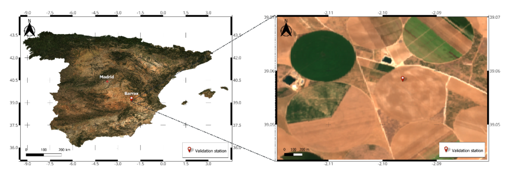
Figure 1: Geographic location of the study area at the “Las Tiesas” farm (Barrax, Albacete), selected for the validation of LST products.
3.2. In-situ data and instrumentation
To retrieve surface temperature data for the study area, measurements were obtained from a fixed radiometric station installed at the site. The dataset covers the period from January 1, 2021 through May 28, 2025.
The station is equipped with a data acquisition system based on Campbell Scientific dataloggers (models CR1000 and CR1000X, depending on the annual campaign). The system records continuous surface temperature values at a sampling interval of 5 minutes, depending on the specific campaign configuration. The instrument employed is a Campbell Scientific IR120 broadband infrared radiometer (8–14 µm), mounted at a height of 4 meters with a nadir view. It points towards a homogeneous surface characterized by bare soil or agricultural crops, depending on the season. This radiometer is periodically calibrated using a LAND P80P calibration source, with an estimated uncertainty of approximately ±0.2 K. The calibrations performed show minimal differences between consecutive checks, indicating radiometric stability.
3.3. Landsat-9 data
This study utilized imagery acquired by the Landsat 9 satellite, launched on September 27, 2021, specifically data from the Thermal Infrared Sensor 2 (TIRS-2). Unlike its predecessor on Landsat 8, TIRS-2 was designed with significant improvements to mitigate the stray light anomaly, thereby enhancing the radiometric stability of the thermal bands (Montanaro et al., 2022). Processing was conducted on the Google Earth Engine (GEE) platform, accessing two distinct datasets within Collection 2 (EROS Center, 2020b), which provide scaled, georeferenced, and sensor-calibrated radiance.
The entire available historical time series over Barrax, starting from October 31, 2021, was processed. A cloud filter was applied, and pixel values corresponding to the coordinates of the Barrax station were extracted.
To implement the proposed Split-Window algorithm, ‘Landsat 9 Collection 2 Tier 1 Level-1 (L1TP)’ products were used, utilizing bands 10 (10.60–11.19 µm) and 11 (11.50–12.51 µm). Although the TIRS-2 sensor acquires data at a native resolution of 100 m, L1TP products are resampled to 30 m by the USGS using cubic convolution to match the bands of the Operational Land Imager 2 (OLI-2) sensor (Eon et al., 2024). Digital numbers were converted to spectral radiance and subsequently to brightness temperature (in Kelvin) at the top-of-atmosphere (TOA), using the radiometric calibration coefficients and thermal constants (K1, K2) provided in the metadata of each scene (EROS Center, 2020a).
Additionally, surface reflectance spectral bands from the Landsat 9 Level-2 Science Product (L2SP) were processed, specifically Band 4 (Red) and Band 5 (Near-Infrared). These atmospherically corrected bands are essential for calculating the Normalized Difference Vegetation Index (NDVI) at the native 30 m resolution, which serves as the input variable for the dynamic estimation of Land Surface Emissivity (LSE) required by the Split-Window algorithm (Eq. 1).
3.4. Atmospheric data (ERA5)
Total column water vapor values, required for the application of the SW algorithm, were obtained from the ERA5 global climate reanalysis dataset, produced by the Copernicus Climate Change Service (C3S) at ECMWF. The ‘ERA5 Hourly – ECMWF Climate Reanalysis’ product, available on Google Earth Engine, was utilized. This dataset provides hourly estimates for a wide range of atmospheric, land, and oceanic climate variables. The data cover the Earth on a ~31 km grid and resolve the atmosphere using 137 levels from the surface up to a height of 80 km (Hersbach et al., 2020), offering an extensive period of availability (from 1940 to the present).
From this product, the ‘total column water vapour’ variable was extracted. This parameter represents the total amount of water vapor in a column extending from the Earth’s surface to the TOA. Accordingly, for each acquired Landsat 9 scene, the ERA5 image corresponding to the nearest hour was selected. Water vapor values, originally in kg/m2, were converted to g/cm2 to ensure consistency with the units required by the Split-Window algorithm coefficients, and were spatially extracted at the exact coordinates of the validation station.
Additionally, the surface downward longwave radiation flux parameter (‘mean_surface_downward_long_wave_radiation_flux’) was extracted. This variable is essential for the rigorous correction of the in-situ radiometer data. It represents the atmospheric thermal irradiance (W/m2), which was temporally interpolated to the exact minute of the station measurement. Subsequently, this flux was converted into equivalent radiative temperature and, through inversion, into downward atmospheric radiance. This step is necessary to isolate the surface’s own emission from the sky reflection captured by the instrument.
4. SW algorithm validation
To assess the accuracy of the proposed Split-Window (SW) algorithm and compare it against the official USGS Level-2 Land Surface Temperature product, a validation based on in-situ radiometric temperature measurements was conducted. Prior to the main validation, a preliminary sensitivity analysis was performed by running the SW algorithm using the emissivity band from the L2 product instead of the locally estimated LSE. This step was intended to discern whether potential improvements in estimation were attributable to the algorithm coefficients or to the emissivity source.
The validation process involved extracting pixel values corresponding to the station location and linearly interpolating the field measurements to the exact satellite overpass time. Scenes affected by cloud contamination were discarded. Quantitative assessment relied on the calculation of standard statistical metrics: Bias, Root Mean Square Error (RMSE), Mean Absolute Error (MAE), and the coefficient of determination (R2).
Furthermore, a graphical error analysis was conducted using scatter plots to assess linearity, time series to verify the seasonal consistency of the data, and residual plots against surface temperature and atmospheric water vapor content to identify potential systematic biases dependent on thermal or atmospheric conditions.
5. Results and discussion
5.1. SW coefficients and sensitivity analysis
The detailed procedure for the retrieval of the SW algorithm coefficients and assessment of uncertainties (sensitivity analysis) can be found in Jiménez-Muñoz & Sobrino (2008). This procedure was also used to develop a SW algorithm for Landsat-8 data (Jiménez-Muñoz et al. 2014).
Basically, SW coefficients involved in Equation (1) were obtained from statistical regression over a database of at-sensor brightness temperatures computed from forward simulations. For this purpose, different atmospheric profiles extracted from the GAPRI database (Mattar et al. 2015) were used as input to the MODTRAN radiative transfer code. MODTRAN atmospheric outputs were combined to a set of surface emissivities extracted from the ECOSTRESS spectral library to reproduce at-sensor brightness temperature values from the radiative transfer equation.
The simulated database was also used to perform the sensitivity analysis of the SW algorithm to the noise equivalent delta temperatures (NEDT) of Landsat-9 TIRS bands, as well as surface emissivity and atmospheric water vapor uncertainties. Table 2 shows the values of the coefficients and also the different contributions to the sensitivity analysis. The mathematical structure given in Eq. (1) is able to fit the simulated database with a standard error of estimation of 0.3 K. Impact of NEDT and water vapor uncertainty is on the same order or even below. The greatest contribution in the sensitivity analysis is due to the surface emissivity uncertainty, of around 1.1 K. Overall, the SW algorithm is expected to provide LST retrievals with RMSE of 1.2 K. Substituting these derived coefficients into the general structure yields the specific SW algorithm for Landsat-9 (Eq. 3):
Table 3: Split-window coefficients (see Eq. 3) and contributions to the sensitivity analysis. ‘St dev’ is the standard error of estimation and ‘r’ the linear (Pearson) correlation coefficient obtained in the statistical regression. Uncertainties due to NEDT of Landsat-9 TIRS bands (unoise), surface emissivity (uemis) and total atmospheric water vapor content (uwv) are also provided. The Root Mean Square Error (RMSE) provides the overall accuracy of the SW algorithm.
| Coefficients | St dev [K] | r | unoise [K] | uemis [K] | uwv [K] | RMSE [K] | |
| c0 =0.0559 c1 =1.3477 c2 =0.1458 c3 =52.577 | c4 = -3.728 c5 -111.753 c6 =17.066 | 0.3 | 0.988 | 0.3 | 1.1 | 0.12 | 1.2 |
5.2. In-situ Land Surface Temperature retrieval
The data acquired by the infrared radiometer correspond to brightness temperature, representing the integration of incident radiation upon the sensor within its specific spectral bandwidth. Given the sensor’s low installation height above the canopy (< 5 m), a simplified version of the Radiative Transfer Equation (RTE) was applied. Due to the short optical path length between the surface and the sensor, atmospheric transmittance is considered unitary, and the upwelling atmospheric emission from the intermediate air layer is assumed to be negligible. Under these proximal sensing conditions, the radiance measured by the sensor (Lsen) is defined exclusively as the sum of the surface thermal emission and the reflection of the downwelling atmospheric irradiance, both integrated over the sensor’s spectral response function:
where λ is the wavelength, f(λ) is the instrument’s spectral response function, Bλ(Ts) is the spectral radiance emitted by a blackbody at temperature Ts according to Planck’s law, (ελ) represents the spectral surface emissivity, and L↓atm,λ denotes the spectral downwelling atmospheric irradiance.
The brightness temperature was derived by integrating the instrument’s spectral response function with Planck’s Law. The downwelling irradiance component was retrieved from the ERA5 product, temporally interpolated to match the exact acquisition time of the radiometer. Since ERA5 provides broadband downward longwave radiation flux, estimating its specific contribution within the radiometer’s spectral range was necessary. To achieve this, the effective sky brightness temperature was first calculated assuming blackbody behavior according to the Stefan-Boltzmann Law. Subsequently, this temperature was converted into in-band radiance by applying Planck’s Law convolved with the sensor’s spectral response function, maintaining the strict spectral dependence λ of the atmospheric emission.
Surface emissivity was estimated dynamically using the NDVITHM, following the mathematical framework previously described in Section 2.1. However, for its implementation in the broadband radiometer correction, Sentinel-2 data were used, specifically the Surface Reflectance product (Level-2A); its 10 m spatial resolution allows for a rigorous characterization of sub-pixel heterogeneity within the radiometer’s FOV, thereby minimizing scaling errors compared to coarser resolution sensors. Based on the interpolated Sentinel-2 NDVI time series, vegetation fractional cover and emissivity were computed using the specific thresholds for bare soil (NDVIs=0.2; εs=0.97), derived from previous CIMEL measurements conducted to characterize the Barrax soil, and dense vegetation (NDVIv=0.9; εv=0.99) in the Barrax area (Sobrino & Raissouni, 2000; Sobrino et al., 2008), incorporating a cavity correction term of 0.005. These effective values are treated as the band-integrated emissivity ε.
This approach enabled the generation of a continuous emissivity time series coupled to the actual phenological evolution of the crop. This series was subsequently used to invert the Radiative Transfer Equation, correcting the in-situ measurements for atmospheric reflection effects. Finally, the surface emission term in Equation (4) was isolated, and Planck’s function—convolved with the sensor’s spectral response function—was inverted to retrieve the in-situ Land Surface Temperature (Ts), corrected for both emissivity and downwelling sky irradiance.
5.3. SW algorithm testing
To validate the proposed SW algorithm (Eq. 3), the retrieved LST values—spatiotemporally coincident with the validation station records—were compared at the exact satellite overpass time, excluding cloud-contaminated scenes. Subsequently, a linear regression analysis was performed between both datasets, and various statistical metrics were calculated for a quantitative assessment across the entire dataset of 43 valid processed images (N=43). This validation was conducted for the proposed SW algorithm, the SW algorithm computed using the L2 emissivity product, and the official temperature product provided by the USGS (L2).
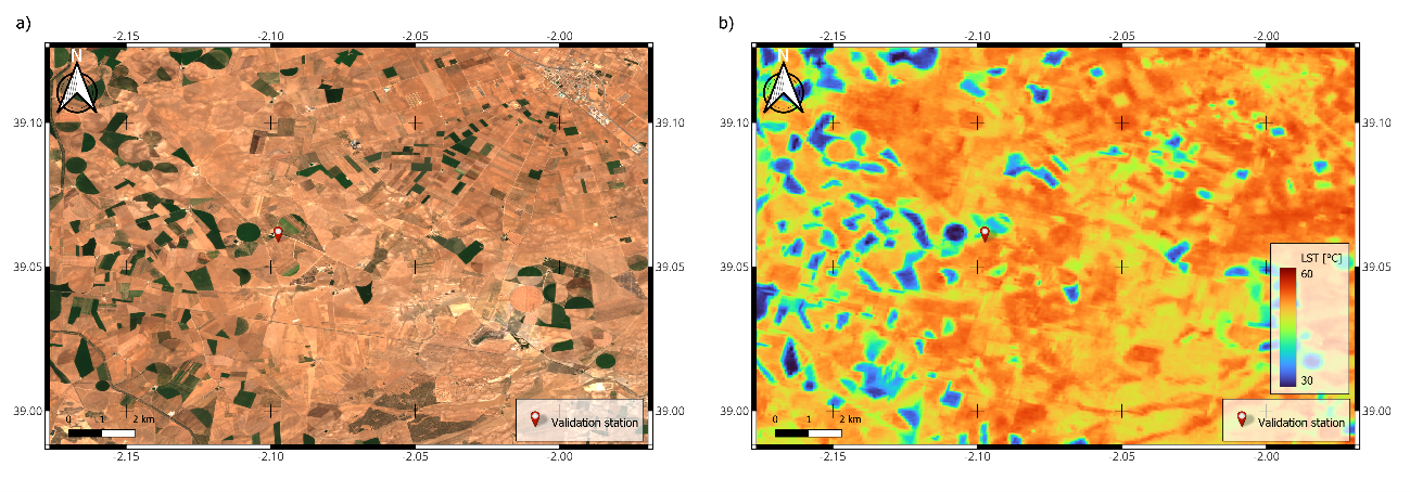
Prior to the point-based statistical validation, a qualitative assessment of the spatial coherence of the LST estimates generated by the proposed Split-Window algorithm was conducted. Figure 2 compares the true-color (RGB) image with the retrieved LST map. A precise spatial correspondence between land cover patterns and thermal distribution is observed. Center-pivot irrigation fields, clearly identifiable by their high green reflectance and circular shape in the RGB image, coincide perfectly with areas of lower temperature (blue tones in the thermal map), due to the cooling effect of crop evapotranspiration. Conversely, areas of bare soil and dry vegetation exhibit the highest temperatures (reddish tones), exceeding 50 °C. This spatial coherence confirms that the algorithm, coupled with the Sentinel-2-based emissivity correction, correctly discriminates the thermal heterogeneity of the agricultural landscape without introducing significant noise.
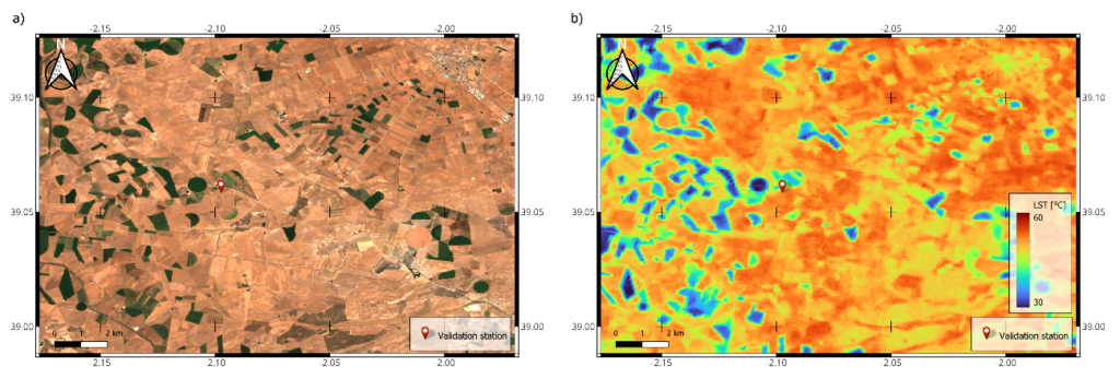
Figure 2. Spatial representation of the study area in Barrax (Albacete) for the date 24-08-2024. (a) True-color (RGB) composite image showing crop heterogeneity and center-pivot irrigation systems. (b) Land Surface Temperature (LST) map generated using the proposed Split-Window algorithm. The red marker indicates the exact location of the validation station.
The quantitative comparison between the results obtained with the emissivity calculated via the proposed methodology and those derived using the emissivity from the L2 product is presented in Table 3. The differences between using the NDVI-derived emissivity and the official product emissivity (∆RMSE) are lower than 0.05 °C, which demonstrates the robustness and insensitivity to the applied threshold.
Figure 3 illustrates the comparison between the values obtained with the proposed algorithm and those provided by the USGS L2 product against the in-situ measurements. As detailed in Table 3, the proposed Split-Window algorithm, utilizing the specific coefficients and a local NDVI-derived emissivity, achieved an RMSE of 1.22 °C, reflecting the high accuracy of the algorithm under local conditions.
In contrast, although the official L2 product exhibits a high correlation (R2=0.991), it presents a systematic positive bias (+1.15 °C) and a significantly higher RMSE (1.99 °C). This discrepancy is also evident in the error dispersion: while the proposed algorithm maintains a lower standard deviation of the residuals (1.16 °C), the official product shows greater dispersion (1.63 °C). This suggests that the USGS global atmospheric or emissivity correction introduces additional uncertainty over these types of agricultural land covers.
Table 3. Statistical metrics obtained from the validation of Landsat 9 LST estimates against in-situ measurements (N=43).
| RMSE [°C] | Bias [°C] | MAE [°C] | Std [°C] | R2 | |
| Proposed SW | 1.22 | -0.35 | 1.03 | 1.16 | 0.995 |
| SW (using the L2 emissivity product) | 1.26 | -0.48 | 1.05 | 1.17 | 0.995 |
| Official USGS product | 1.99 | 1.15 | 1.53 | 1.63 | 0.991 |
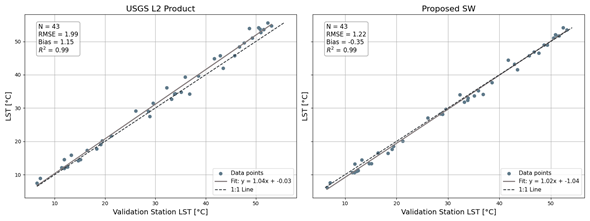
Figure 3.Validation of Landsat 9 estimated LST against in-situ radiometric measurements (N=43). (a) Comparison of the USGS Level-2 operational product (left). (b) Comparison of the proposed Split-Window algorithm (right). The dashed line represents the 1:1 relationship, while the solid line indicates the linear regression fit of the data. Statistical accuracy metrics (RMSE, Bias, and R2) are displayed in the upper-left inset of each plot.
Figure 4 displays the temporal evolution of the LST series, revealing high radiometric consistency between the proposed SW estimates and the station measurements throughout the entire study period. The algorithm faithfully reproduces seasonal variability, accurately capturing both summer maxima and winter minima. Notably, the time series of the proposed algorithm aligns with the station baseline, effectively correcting the offset or constant positive bias visually observed in the official USGS product series.
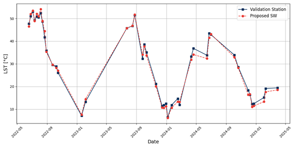
Figure 4. Temporal evolution of LST at the validation site during the study period (2022–2025). The solid blue line represents in-situ measurements (Validation Station), while the dashed red line indicates the estimates from the proposed Split-Window algorithm (Proposed SW).
Additionally, Figures 5 and 6 present the temperature residuals (LSTSW-LSTstation) as a function of station temperature and ERA5 water vapor content, respectively. In the temperature analysis (Fig. 5), the scatter plot shows a distribution centered around zero—consistent with the low bias of -0.35 °C—and a uniform dispersion across the entire thermal range. This confirms the homoscedasticity of the error; that is, the algorithm operates with consistent precision at both low and high temperatures. The dashed lines represent the 95% confidence interval (±2 RMSE). Points falling within these limits are considered within the expected statistical uncertainty, while those outside could be attributed to isolated anomalies or outliers. In this case, only 2 points were identified outside this interval, corresponding to 4.7% of the data. This percentage is fully consistent with a normal distribution of errors, thus ruling out systematic issues within the model.
Finally, regarding water vapor (Fig. 6), the residuals exhibit independence from the atmospheric moisture load. The absence of trends or biases on days with high water vapor concentrations demonstrates the robustness of the Split-Window coefficients in effectively correcting for differential atmospheric absorption, thereby overcoming the typical limitations of Single-Channel (SC) algorithms under humid conditions (Jiménez-Muñoz et al., 2014).
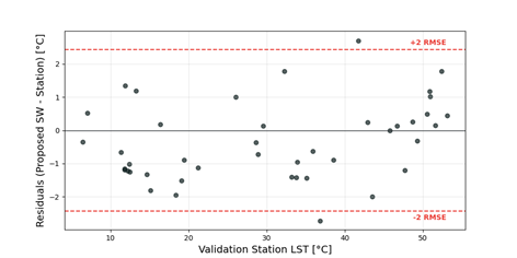
Figure 5. Distribution of temperature residuals (LSTSW-LSTstation) versus in-situ surface temperature.
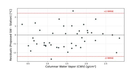
Figure 6. Distribution of temperature residuals (LSTSW-LSTstation) versus Columnar Water Vapor (CWV).
6. Conclusions
This study proposes and evaluates a Split-Window (SW) algorithm based on global coefficients for Land Surface Temperature (LST) retrieval using data from the TIRS-2 sensor onboard Landsat 9. Comprehensive validation against continuous radiometric measurements at the Barrax agricultural station demonstrated the viability and high fidelity of the proposed method. Quantitatively, the SW algorithm yielded a Root Mean Square Error (RMSE) of 1.22 °C and a near-zero bias of -0.35 °C.
This level of accuracy is consistent with existing literature regarding LST retrieval without in-situ atmospheric data. Specifically, previous simulations for TIRS sensors indicate that Split-Window algorithms typically exhibit errors below 1.5 °C, outperforming Single-Channel (SC) methods under variable humidity conditions (Jiménez-Muñoz et al., 2014). Furthermore, these results fall within the expected uncertainty range for algorithms that do not require concurrent radiosoundings, as historical performance across the Landsat series typically ranges between 0.9 °C and 2.0 °C, depending on the method and water vapor load (Sobrino et al., 2004; Jiménez-Muñoz & Sobrino, 2008). Therefore, the obtained RMSE of 1.22 °C validates the global parameterization employed and confirms its operational suitability.
Comparison with the official USGS Level-2 (L2) product revealed a substantial methodological improvement, as the operational product exhibited a significant systematic overestimation (+1.15 °C) and a considerably higher RMSE (1.99 °C) over the same time series. This discrepancy underscores the limitations of general-purpose operational algorithms in phenologically dynamic agricultural areas and highlights the added value of coupling LST retrieval with a local emissivity estimation derived from simultaneous optical bands via the NDVI Threshold Method. Additionally, residual analysis confirmed the stability of the proposed model, demonstrating that its predictive performance does not degrade under extreme thermal conditions or variations in columnar atmospheric water vapor content. In conclusion, the Split-Window formulation validated in this study constitutes a robust, accurate, and independent approach, making it highly recommended for agronomic applications and energy balance studies requiring high-spatial-resolution thermal data.
Autor Contributions
José A. Sobrino: Funding acquisition, Project administration, Resources, Supervision, Investigation, Conceptualization, Methodology, Writing – Review & Editing. Sergio Gimeno: Methodology, Software, Validation, Formal analysis, Investigation, Data Curation, Writing – Original Draft. Juan Carlos Jiménez-Muñoz and Drazen Skokovic: Investigation, Sotfware, Conceptualization, Methodology, Writing – Review & Editing.
Declaration of Competing Interest
The authors declare that they have no known competing financial interests or personal relationships that could have appeared to influence the work reported in this paper.
Acknowledgments
The authors thank the associate editor and the reviewers for their systematic review and valuable comments.
Funding
This research was funded by the European Union and the Government of the Valencian Community through the project “Indicadores medioambientales y fenómenos adversos en la Comunidad Valenciana usando datos de satélite,” under the PROMETEO 2023 funding programme (CIPROM/2023/42), and by Project PID2023-150737OB-I00, funded by MICIU/AEI/10.13039/501100011033 and by FEDER, EU.
References
Baldridge, A., Hook, S., Grove, C., & Rivera, G. (2009). The ASTER spectral library version 2.0. Remote Sensing Of Environment, 113(4), 711-715. https://doi.org/10.1016/j.rse.2008.11.007
Coll, C., Garcia-Santos, V., Niclos, R., & Caselles, V. (2016). Test of the MODIS Land Surface Temperature and Emissivity Separation Algorithm With Ground Measurements Over a Rice Paddy. IEEE Transactions On Geoscience And Remote Sensing, 54(5), 3061-3069. https://doi.org/10.1109/tgrs.2015.2510426
Crawford, C. J., Roy, D. P., Arab, S., Barnes, C., Vermote, E., Hulley, G., Gerace, A., Choate, M., Engebretson, C., Micijevic, E., Schmidt, G., Anderson, C., Anderson, M., Bouchard, M., Cook, B., Dittmeier, R., Howard, D., Jenkerson, C., Kim, M., . . . Zahn, S. (2023). The 50-year Landsat collection 2 archive. Science Of Remote Sensing, 8, 100103. https://doi.org/10.1016/j.srs.2023.100103
Earth Resources Observation and Science (EROS) Center. (2020a). Landsat 8-9 Operational Land Imager / Thermal Infrared Sensor Level-1, Collection 2 [dataset]. U.S. Geological Survey. https://doi.org/10.5066/P975CC9B
Earth Resources Observation and Science (EROS) Center. (2020b). Landsat 8-9 Operational Land Imager / Thermal Infrared Sensor Level-2, Collection 2 [dataset]. U.S. Geological Survey. https://doi.org/10.5066/P9OGBGM6
Eon, R., Wenny, B. N., Poole, E., Kay, S. E., Montanaro, M., Gerace, A., & Thome, K. J. (2024). Landsat 9 Thermal Infrared Sensor-2 (TIRS-2) Pre- and Post-Launch Spatial Response Performance. Remote Sensing, 16(6), 1065. https://doi.org/10.3390/rs16061065
Hersbach, H., Bell, B., Berrisford, P., Hirahara, S., Horányi, A., Muñoz‐Sabater, J., Nicolas, J., Peubey, C., Radu, R., Schepers, D., Simmons, A., Soci, C., Abdalla, S., Abellan, X., Balsamo, G., Bechtold, P., Biavati, G., Bidlot, J., Bonavita, M., . . . Thépaut, J. (2020). The ERA5 global reanalysis. Quarterly Journal Of The Royal Meteorological Society, 146(730), 1999-2049. https://doi.org/10.1002/qj.3803
Jimenez-Munoz, J. C., Sobrino, J. A., Skokovic, D., Mattar, C., & Cristobal, J. (2014). Land surface temperature retrieval methods from LANDSAT-8 Thermal Infrared Sensor data. IEEE Geoscience And Remote Sensing Letters, 11(10), 1840-1843. https://doi.org/10.1109/lgrs.2014.2312032
Jimenez-Munoz, J., & Sobrino, J. A. (2008). Split-Window Coefficients for Land Surface Temperature Retrieval From Low-Resolution Thermal Infrared Sensors. IEEE Geoscience And Remote Sensing Letters, 5(4), 806-809. https://doi.org/10.1109/lgrs.2008.2001636
Mattar, C., Durán-Alarcón, C., Jiménez-Muñoz, J. C., Santamaría-Artigas, A., Olivera-Guerra, L., & Sobrino, J. A. (2015). Global Atmospheric Profiles from Reanalysis Information (GAPRI): a new database for earth surface temperature retrieval. International Journal Of Remote Sensing, 36(19-20), 5045-5060. https://doi.org/10.1080/01431161.2015.1054965
Meng, X., & Cheng, J. (2018). Evaluating Eight Global Reanalysis Products for Atmospheric Correction of Thermal Infrared Sensor—Application to Landsat 8 TIRS10 Data. Remote Sensing, 10(3), 474. https://doi.org/10.3390/rs10030474
Montanaro, M., McCorkel, J., Tveekrem, J., Stauder, J., Mentzell, E., Lunsford, A., Hair, J., & Reuter, D. (2022). Landsat 9 Thermal Infrared Sensor 2 (TIRS-2) Stray Light Mitigation and Assessment. IEEE Transactions On Geoscience And Remote Sensing, 60, 1-8. https://doi.org/10.1109/tgrs.2022.3177312
Peres, L. F., Sobrino, J. A., Libonati, R., Jiménez‐Muñoz, J. C., Dacamara, C. C., & Romaguera, M. (2008). Validation of a temperature emissivity separation hybrid method from airborne hyperspectral scanner data and ground measurements in the SEN2FLEX field campaign. International Journal Of Remote Sensing, 29(24), 7251-7268. https://doi.org/10.1080/01431160802036532
Skokovic, D., Sobrino, J. A., & Jimenez-Munoz, J. C. (2016). Vicarious Calibration of the Landsat 7 Thermal Infrared Band and LST Algorithm Validation of the ETM+ Instrument Using Three Global Atmospheric Profiles. IEEE Transactions On Geoscience And Remote Sensing, 55(3), 1804-1811. https://doi.org/10.1109/tgrs.2016.2633810
Sobrino, J. A., Jimenez-Munoz, J. C., Soria, G., Romaguera, M., Guanter, L., Moreno, J., Plaza, A., & Martinez, P. (2008). Land Surface Emissivity Retrieval From Different VNIR and TIR Sensors. IEEE Transactions On Geoscience And Remote Sensing, 46(2), 316-327. https://doi.org/10.1109/tgrs.2007.904834
Sobrino, J. A., Jiménez-Muñoz, J. C., & Paolini, L. (2004). Land surface temperature retrieval from LANDSAT TM 5. Remote Sensing Of Environment, 90(4), 434-440. https://doi.org/10.1016/j.rse.2004.02.003
Sobrino, J. A., Li, Z., Stoll, M. P., & Becker, F. (1996). Multi-channel and multi-angle algorithms for estimating sea and land surface temperature with ATSR data. International Journal Of Remote Sensing, 17(11), 2089-2114. https://doi.org/10.1080/01431169608948760
Sobrino, J. A., & Raissouni, N. (2000). Toward remote sensing methods for land cover dynamic monitoring: Application to Morocco. International Journal Of Remote Sensing, 21(2), 353-366. https://doi.org/10.1080/014311600210876
Sobrino, J. A., & Skoković, D. (2016). Permanent Stations for Calibration/Validation of Thermal Sensors over Spain. Data, 1(2), 10. https://doi.org/10.3390/data1020010
U.S. Geological Survey, 2021, Landsat Collection 2 Level-2 Science Products: U.S. Geological Survey Fact Sheet 2021–3055, 2 p., https://doi.org/10.3133/fs20213055.
Wan, Z., & Dozier, J. (1996). A generalized split-window algorithm for retrieving land-surface temperature from space. IEEE Transactions On Geoscience And Remote Sensing, 34(4), 892-905. https://doi.org/10.1109/36.508406
Zhou, S., & Cheng, J. (2020). An Improved Temperature and Emissivity Separation Algorithm for the Advanced Himawari Imager. IEEE Transactions On Geoscience And Remote Sensing, 58(10), 7105-7124. https://doi.org/10.1109/tgrs.2020.2979846
Publisher’s Note
The statements, opinions and data contained in all publications are solely those of the individual author(s) and contributor(s) and not of Recent Advances S.L. and/or the editor(s). Recent Advances S.L. and/or the editor(s) disclaim responsability for any injury to people or property resulting from any ideas, methods, instructions or products referred to in the content.